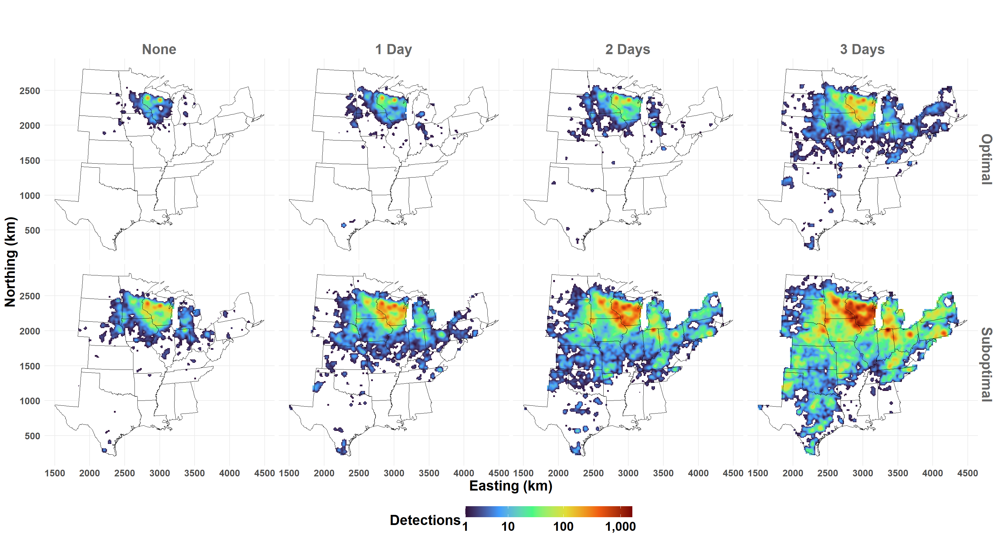
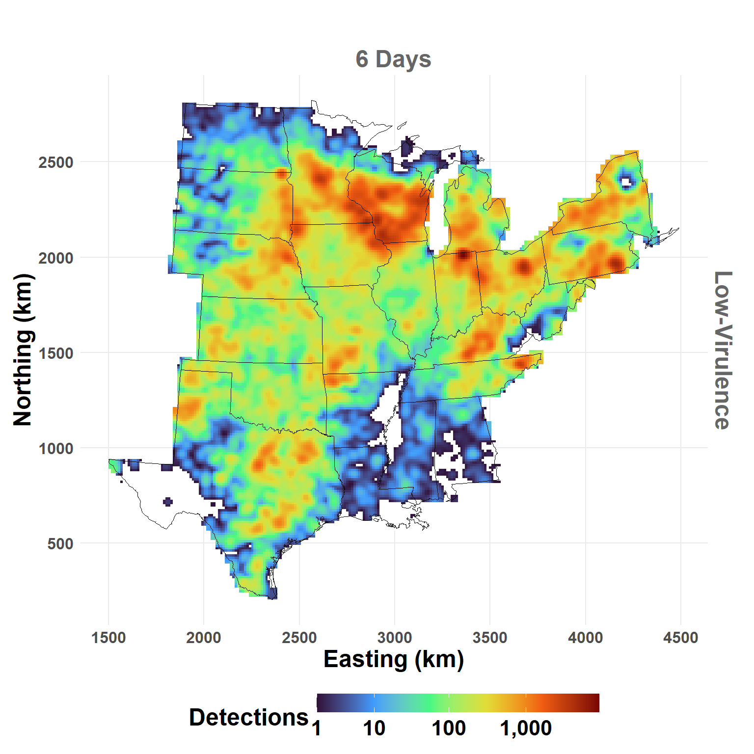
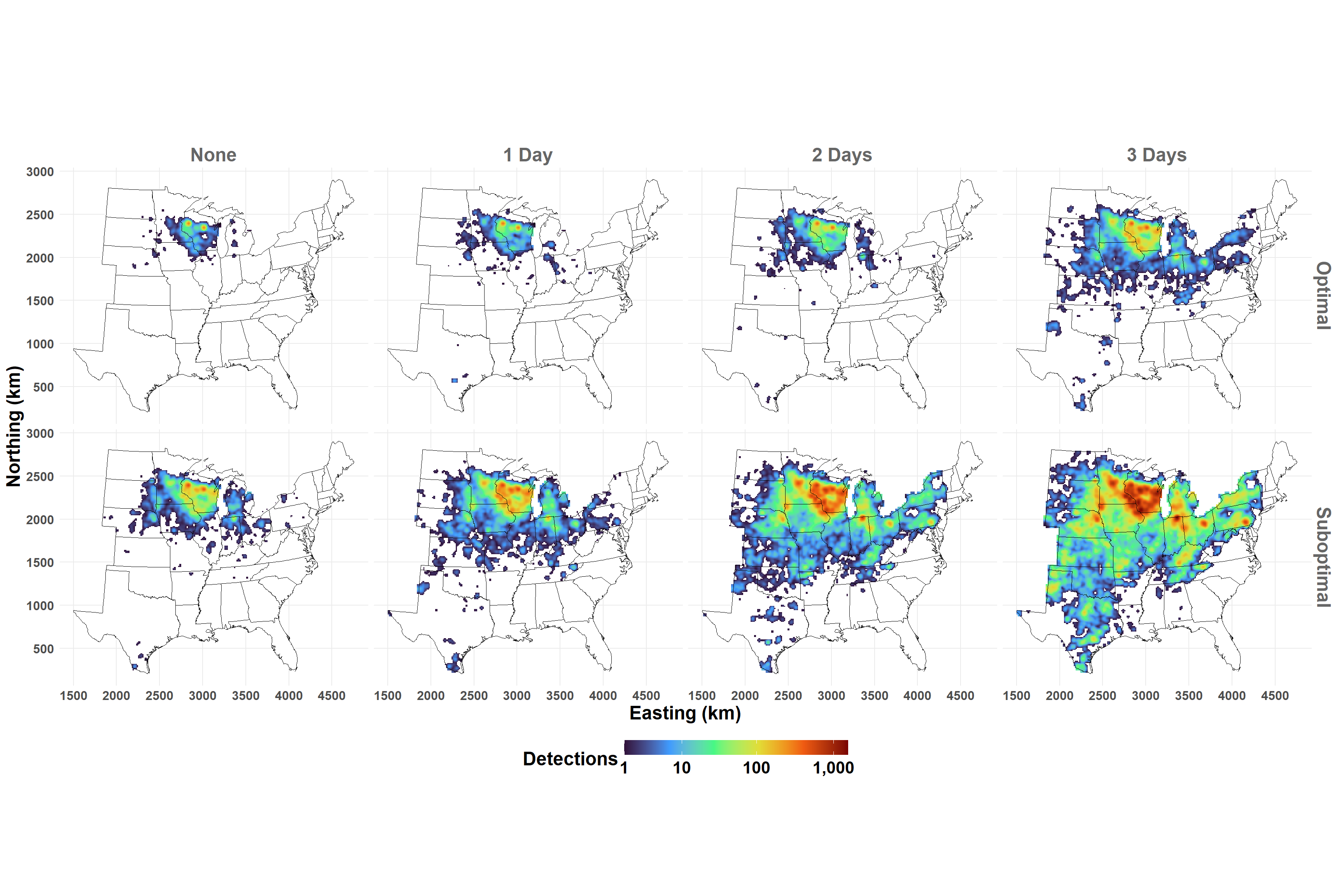
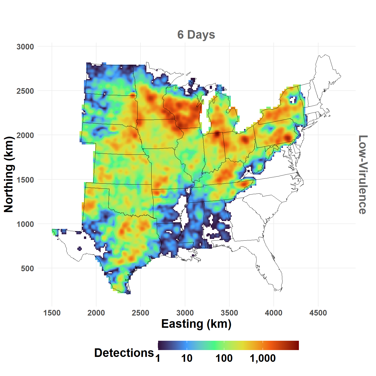
Map cumulative case detections across all iterations by scenario
Central U.S. Maps
Prepare to plot outbreak maps for the central region. First, get shapefile for the conterminous U.S. and set state boundaries for regional scenario. Then, create a raster grid version.
Region Boundaries
Get shapefile and subset to region
Code
## Get shapefile for conterminous U.S.whole_us <-vect(here("script-inputs/shapefile/Contiguous_USA_for Regional_Model.shp")) ## Boundaries for Central U.S.central_states <-c("Alabama", "Arkansas", "Illinois", "Indiana", "Iowa", "Kansas", "Kentucky", "Louisiana", "Michigan", "Minnesota", "Mississippi", "Missouri", "Nebraska", "New York", "North Dakota", "Ohio", "Oklahoma", "Pennsylvania", "South Dakota", "Tennessee", "Texas", "West Virginia", "Wisconsin")central_us <-subset(whole_us, whole_us$STATE_NAME %in% central_states)
Create Raster Grid
Create a raster grid version for the central region
Code
tmp_r <-rast(ext(central_us), resolution =25000, # 25km gridcrs =crs(central_us))central_r <-rasterize(central_us, tmp_r)central_r[central_r ==1] <-0# set land areas to 0
Count Cumulative Case Detections
raster_point_counts() will count the number of detection events in each 25km cell. Smoothing the raster will improve the appearance by making the cells smaller and finding averages of surrounding cells.
Create a raster grid version for the eastern region
Code
tmp_r <-rast(ext(eastern_us), resolution =25000, # 25km gridcrs =crs(eastern_us))east_r <-rasterize(eastern_us, tmp_r)east_r[east_r ==1] <-0# set land areas to 0
Count Cumulative Case Detections
raster_point_counts() will count the number of detection events in each 25km cell. Smoothing the raster will improve the appearance by making the cells smaller and finding averages of surrounding cells.