Infection Summary
summarize_infections() summarizes infection metrics by iteration.
Code
## Summarize infection metrics for each iteration <- summarize_infections (infection)
View a subset of infect_summary
Code
## Filter data to scenario <- infect_summary %>% filter (region == "central" ) %>% filter (scenario_type == "suboptimal" ) %>% filter (preclinical == 2 )## Select and order columns to display <- infect_summary_select[c ("iteration" , "farms_infected" , "cattle_infected" , "first_infect" , "last_infect" )]<- infect_summary_select %>% mutate (across (c ("iteration" , "farms_infected" , "cattle_infected" , "first_infect" , "last_infect" ), comma))## Check data head (infect_summary_select)
1
82
18,980
10
54
2
13
4,893
10
27
3
179
51,364
10
85
4
10
2,271
10
36
5
20
6,115
10
42
6
116
54,607
10
111
Summary Statistics
generate_infect_statistics() returns summary statistics for each modeling scenario. Results are grouped by region, scenario_type, and preclinical. The output is filtered by summary and region to compare farms_infected and cattle_infected between scenarios.
Code
<- generate_infect_statistics (infect_summary)## Filter to farms <- infect_config_summary %>% filter (summary == "farms_infected" )## Filter to cattle <- infect_config_summary %>% filter (summary == "cattle_infected" )
Infected Farms
The number of infected farms
Code
## Filter to western region <- farms_inf_summary %>% filter (region == "western" )## Select and order columns <- farms_western_summary[c ("scenario_type" , "preclinical" , "mean" , "q05" , "q25" , "q50" , "q75" , "q95" )]<- farms_western_select %>% mutate_if (is.numeric, round, digits = 2 ) %>% mutate_if (is.numeric, ~ format (.x, nsmall = 2 , big.mark = "," ))
optimal
0
8.29
2.00
3.00
4.00
8.00
31.10
optimal
1
16.63
2.00
4.00
7.00
18.00
66.00
optimal
2
34.95
2.00
5.75
14.00
45.25
150.10
optimal
3
60.04
3.00
8.00
26.00
88.50
212.15
suboptimal
0
47.28
4.00
12.00
30.00
65.00
137.20
suboptimal
1
92.23
6.00
25.00
58.00
135.25
267.05
suboptimal
2
159.91
8.00
43.00
114.50
235.25
461.05
suboptimal
3
303.24
19.90
107.75
237.50
423.25
800.00
low-virulence
6
1,567.76
155.85
725.75
1,449.50
2,288.00
3,455.30
Code
## Filter to western region <- farms_inf_summary %>% filter (region == "central" )## Select and order columns <- farms_central_summary[c ("scenario_type" , "preclinical" , "mean" , "q05" , "q25" , "q50" , "q75" , "q95" )]<- farms_central_select %>% mutate_if (is.numeric, round, digits = 2 ) %>% mutate_if (is.numeric, ~ format (.x, nsmall = 2 , big.mark = "," ))
optimal
0
7.35
2.00
2.00
3.00
6.00
20.05
optimal
1
12.71
2.00
3.00
5.00
11.00
56.00
optimal
2
23.37
2.00
4.00
9.00
22.00
94.00
optimal
3
72.51
3.00
7.00
15.50
67.00
372.35
suboptimal
0
46.92
4.00
9.00
22.00
55.25
176.05
suboptimal
1
106.39
6.00
15.00
41.00
140.25
408.15
suboptimal
2
250.57
7.00
24.00
81.00
369.75
939.20
suboptimal
3
578.08
9.00
45.75
312.50
1,008.25
1,729.50
low-virulence
6
3,722.94
1,491.70
3,034.50
3,917.00
4,595.00
5,520.00
Code
## Filter to eastern region <- farms_inf_summary %>% filter (region == "eastern" )## Select and order columns <- farms_eastern_summary[c ("scenario_type" , "preclinical" , "mean" , "q05" , "q25" , "q50" , "q75" , "q95" )]<- farms_eastern_select %>% mutate_if (is.numeric, round, digits = 2 ) %>% mutate_if (is.numeric, ~ format (.x, nsmall = 2 , big.mark = "," ))
optimal
0
6.56
2.00
2.00
4.00
7.00
20.05
optimal
1
13.59
2.00
3.00
6.00
13.00
57.05
optimal
2
30.40
2.00
5.00
10.00
26.00
124.05
optimal
3
54.78
2.00
7.00
15.00
61.25
237.10
suboptimal
0
41.67
4.00
10.00
21.00
51.00
134.05
suboptimal
1
89.45
5.00
16.00
41.00
94.75
330.70
suboptimal
2
186.16
6.00
26.00
74.00
268.25
684.10
suboptimal
3
457.09
9.00
43.00
250.50
655.50
1,620.15
low-virulence
6
3,101.59
61.85
2,435.75
3,412.50
4,187.25
4,993.10
Total Cattle
The total number of cattle on infected farms
Code
## Filter to western region <- cattle_inf_summary %>% filter (region == "western" )## Select and order columns <- cattle_western_summary[c ("scenario_type" , "preclinical" , "mean" , "q05" , "q25" , "q50" , "q75" , "q95" )]<- cattle_western_select %>% mutate (across (c (mean, q05, q25, q50, q75, q95), comma))
optimal
0
26,882
4,332
4,348
5,286
25,412
127,976
optimal
1
52,327
4,332
4,562
15,731
72,506
208,088
optimal
2
98,475
4,332
6,841
46,188
157,810
322,540
optimal
3
152,194
4,408
16,035
85,879
243,585
464,729
suboptimal
0
131,046
5,026
27,389
96,664
201,537
362,921
suboptimal
1
218,642
5,972
68,208
182,701
327,252
560,498
suboptimal
2
347,062
10,812
123,388
277,594
472,179
872,234
suboptimal
3
572,168
45,177
244,216
457,094
765,672
1,445,881
low-virulence
6
2,782,496
266,320
1,041,360
2,119,552
4,499,446
6,416,444
Code
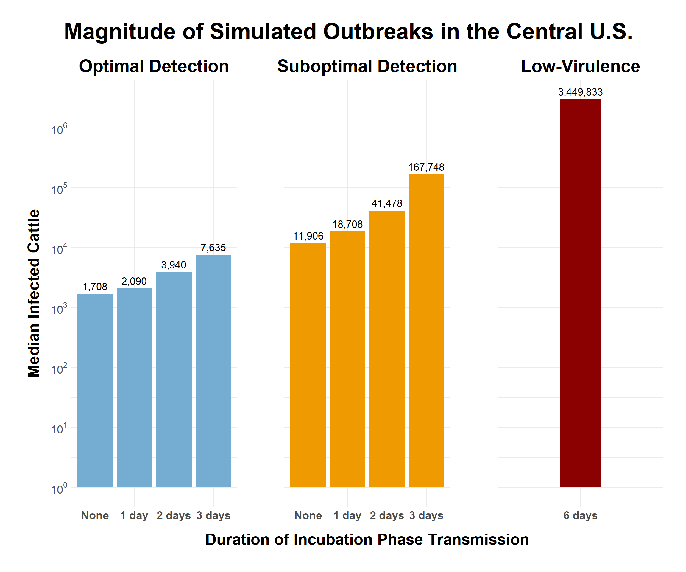
## Filter to central region <- cattle_inf_summary %>% filter (region == "central" )## Select and order columns <- cattle_central_summary[c ("scenario_type" , "preclinical" , "mean" , "q05" , "q25" , "q50" , "q75" , "q95" )]<- cattle_central_select %>% mutate (across (c (mean, q05, q25, q50, q75, q95), comma))
optimal
0
4,347
1,627
1,627
1,708
2,899
13,059
optimal
1
7,215
1,627
1,676
2,090
6,008
30,945
optimal
2
13,340
1,627
1,804
3,940
11,030
51,068
optimal
3
44,454
1,652
2,390
7,635
33,766
233,235
suboptimal
0
25,980
1,756
4,074
11,906
28,268
103,639
suboptimal
1
62,846
1,873
7,052
18,708
72,517
275,944
suboptimal
2
156,363
2,106
10,802
41,478
201,033
666,540
suboptimal
3
455,723
2,608
20,375
167,748
666,591
1,930,263
low-virulence
6
3,243,922
913,215
2,260,734
3,449,833
4,241,387
5,265,010
Code
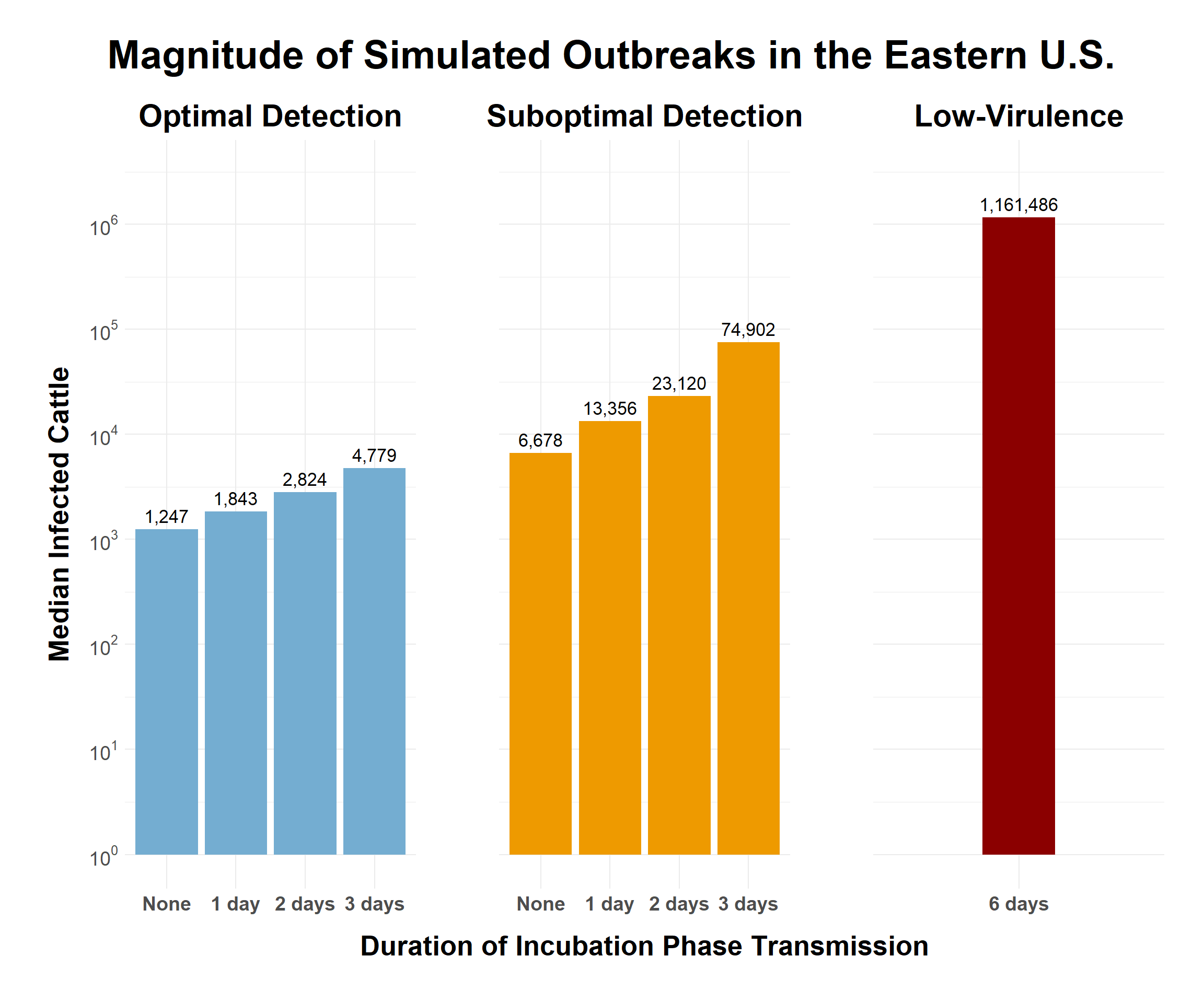
## Filter to eastern region <- cattle_inf_summary %>% filter (region == "eastern" )## Select and order columns <- cattle_eastern_summary[c ("scenario_type" , "preclinical" , "mean" , "q05" , "q25" , "q50" , "q75" , "q95" )]<- cattle_eastern_select %>% mutate (across (c (mean, q05, q25, q50, q75, q95), comma))
optimal
0
2,687
1,164
1,164
1,247
2,236
8,903
optimal
1
5,315
1,164
1,209
1,843
4,832
21,955
optimal
2
11,115
1,164
1,356
2,824
8,958
47,171
optimal
3
17,873
1,164
1,767
4,779
21,290
79,301
suboptimal
0
16,143
1,268
2,524
6,678
18,888
57,100
suboptimal
1
31,848
1,453
4,203
13,356
33,844
126,666
suboptimal
2
62,893
1,606
6,739
23,120
83,049
253,791
suboptimal
3
153,263
1,933
13,766
74,902
215,762
601,651
low-virulence
6
1,019,391
14,089
799,123
1,161,486
1,366,618
1,600,988
Significance Test
Perform significance testing on optimal and suboptimal detection scenarios.
Code
## Filter out low virulence scenarios <- infection %>% filter (scenario_type != "low-virulence" )<- summarize_infections (no_LV)
Linear Model
Code
## Filter to western region <- no_LV_summary %>% filter (region == "western" )<- lm (log (cattle_infected) ~ preclinical * scenario_type, data = no_LV_western_summary)summary (model_western_cattle)
Call:
lm(formula = log(cattle_infected) ~ preclinical * scenario_type,
    data = no_LV_western_summary)

Residuals:
    Min      1Q  Median      3Q     Max
-4.4149 -0.9527  0.1667  1.0284  3.4413

Coefficients:
                             Estimate Std. Error t value Pr(>|t|)
(Intercept)                  10.21850    0.04302 237.527   <2e-16 ***
preclinical1                  0.59910    0.06084   9.847   <2e-16 ***
preclinical2                  1.18004    0.06084  19.396   <2e-16 ***
preclinical3                  1.70577    0.06084  28.037   <2e-16 ***
scenario_type.L               1.26145    0.06084  20.734   <2e-16 ***
preclinical1:scenario_type.L  0.05175    0.08604   0.601    0.548
preclinical2:scenario_type.L -0.07861    0.08604  -0.914    0.361
preclinical3:scenario_type.L  0.02548    0.08604   0.296    0.767
---
Signif. codes:  0 '***' 0.001 '**' 0.01 '*' 0.05 '.' 0.1 ' ' 1

Residual standard error: 1.36 on 3992 degrees of freedom
Multiple R-squared:  0.3943,    Adjusted R-squared:  0.3933
F-statistic: 371.3 on 7 and 3992 DF,  p-value: < 2.2e-16
Code
## Filter to central region <- no_LV_summary %>% filter (region == "central" )<- lm (log (cattle_infected) ~ preclinical * scenario_type, data = no_LV_central_summary)summary (model_central_cattle)
Call:
lm(formula = log(cattle_infected) ~ preclinical * scenario_type,
    data = no_LV_central_summary)

Residuals:
    Min      1Q  Median      3Q     Max
-4.2343 -0.8894 -0.2982  1.0457  4.4918

Coefficients:
                             Estimate Std. Error t value Pr(>|t|)
(Intercept)                   8.60372    0.04628 185.898  < 2e-16 ***
preclinical1                  0.46313    0.06545   7.076 1.75e-12 ***
preclinical2                  1.01288    0.06545  15.475  < 2e-16 ***
preclinical3                  1.83846    0.06545  28.088  < 2e-16 ***
scenario_type.L               1.08133    0.06545  16.521  < 2e-16 ***
preclinical1:scenario_type.L  0.19539    0.09256   2.111   0.0348 *
preclinical2:scenario_type.L  0.39906    0.09256   4.311 1.66e-05 ***
preclinical3:scenario_type.L  0.59686    0.09256   6.448 1.27e-10 ***
---
Signif. codes:  0 '***' 0.001 '**' 0.01 '*' 0.05 '.' 0.1 ' ' 1

Residual standard error: 1.464 on 3992 degrees of freedom
Multiple R-squared:  0.4032,    Adjusted R-squared:  0.4022
F-statistic: 385.3 on 7 and 3992 DF,  p-value: < 2.2e-16
Code
## Filter to eastern region <- no_LV_summary %>% filter (region == "eastern" )<- lm (log (cattle_infected) ~ preclinical * scenario_type, data = no_LV_eastern_summary)summary (model_eastern_cattle)
Call:
lm(formula = log(cattle_infected) ~ preclinical * scenario_type,
    data = no_LV_eastern_summary)

Residuals:
    Min      1Q  Median      3Q     Max
-3.7779 -0.8537 -0.2152  0.9186  4.4417

Coefficients:
                             Estimate Std. Error t value Pr(>|t|)
(Intercept)                   8.21104    0.04188 196.060  < 2e-16 ***
preclinical1                  0.47570    0.05923   8.032 1.25e-15 ***
preclinical2                  0.95705    0.05923  16.159  < 2e-16 ***
preclinical3                  1.59329    0.05923  26.901  < 2e-16 ***
scenario_type.L               0.99160    0.05923  16.742  < 2e-16 ***
preclinical1:scenario_type.L  0.10213    0.08376   1.219  0.22280
preclinical2:scenario_type.L  0.21745    0.08376   2.596  0.00947 **
preclinical3:scenario_type.L  0.46956    0.08376   5.606 2.21e-08 ***
---
Signif. codes:  0 '***' 0.001 '**' 0.01 '*' 0.05 '.' 0.1 ' ' 1

Residual standard error: 1.324 on 3992 degrees of freedom
Multiple R-squared:  0.3794,    Adjusted R-squared:  0.3783
F-statistic: 348.6 on 7 and 3992 DF,  p-value: < 2.2e-16
ANOVA
Code
anova (model_western_cattle)
preclinical
3
1624.908557
541.636186
292.6562847
0.0000000
scenario_type
1
3180.762434
3180.762434
1718.6261576
0.0000000
preclinical:scenario_type
3
4.753417
1.584472
0.8561205
0.4631525
Residuals
3992
7388.229011
1.850759
NA
NA
Code
anova (model_central_cattle)
preclinical
3
1873.93075
624.643584
291.61346
0
scenario_type
1
3804.16224
3804.162244
1775.96463
0
preclinical:scenario_type
3
99.43042
33.143473
15.47296
0
Residuals
3992
8550.96743
2.142026
NA
NA
Code
anova (model_eastern_cattle)
preclinical
3
1391.58709
463.862363
264.46615
0e+00
scenario_type
1
2826.86883
2826.868825
1611.70891
0e+00
preclinical:scenario_type
3
61.25672
20.418906
11.64162
1e-07
Residuals
3992
7001.79806
1.753957
NA
NA
Plot Cattle Numbers
plot_infected_cattle() returns a plot with the duration of incubation phase transmission on the x-axis and the median number of infected cattle (log10) on the y-axis.
Code
<- plot_infected_cattle (cattle_central_summary, "central" )
Code
<- plot_infected_cattle (cattle_eastern_summary, "eastern" )