Tessellation

Mesh Construction and Tessellation

Published

May 4, 2026

1 Overview

The script demonstrates spatial discretization of the study area as detailed in the associated manuscript. First, a triangulated mesh is constructed using administrative boundaries and simulated case point locations. Next, natural neighborhoods are defined using Voronoi tessellation around mesh vertices, such that each cell encapsulates the area each vertex. The resulting polygons define the spatial support and associated integration weights for numerical approximation of the spatial point-process model.

Note

This script assumes that supporting data has already been downloaded to a directory called /demo and that NWS case detections have been simulated as described on the Simulation page of this site.

2 Libraries

Load needed libraries and packages.

Show R Code

library(tidyverse) # data wrangling
options(dplyr.summarise.inform = FALSE)
library(here) # directory managment
library(pals) # color palettes
library(osfr) # interact with Open Science Framework (OSF, data repository)
library(terra) # spatial data manipulation
library(sf) # spatial data manipulation
library(spatstat) # spatial data manipulation
library(raster) # spatial data manipulation
select <- dplyr::select # deconflict dplyr w/raster  

# see https://www.r-inla.org/home
# install.packages("INLA",repos=c(getOption("repos"),INLA="https://inla.r-inla-download.org/R/stable"), dep=TRUE)
library(INLA) # mesh construction, inference

3 Custom Functions

Load customized functions.

Show R Code

source(here("R/utilities.R"))
source_dir(here("R"))

4 Spatial Polygons

Read polygons defining jurisdictional boundaries

Show R Code

states_proj <- st_read(here("demo/study_polygons.gpkg"))

Reading layer `study_states' from data source 
  `D:\Github\hominivorax-geostat\demo\study_polygons.gpkg' using driver `GPKG'
Simple feature collection with 492 features and 122 fields
Geometry type: MULTIPOLYGON
Dimension:     XY
Bounding box:  xmin: -4363.574 ymin: -2203.058 xmax: 2962.346 ymax: 2835.693
Projected CRS: +proj=aea +lat_0=20 +lon_0=-75 +lat_1=10 +lat_2=30 +x_0=0 +y_0=0 +datum=WGS84 +units=km +no_defs

Simplify geometry to help define spatial extent of study area.

Show R Code

states_union <- st_union(states_proj) # dissolve states

# explode islands
poly_single <- st_cast(states_union, "POLYGON", warn = FALSE)

# calculate areas
areas <- st_area(poly_single)

# set threshold to remove smaller islands
threshold <- units::set_units(500, km^2)

# remove islands
states_simple <- poly_single[areas > threshold, ]

5 Simulated NWS Cases

These are NWS cases as simulated in the Simulation tab of this site.

Show R Code

sim_data_df <- read_csv(here("demo/sim_locations_demo.csv"))

nws_points <- vect(sim_data_df, geom = c("x", "y"), crs = "EPSG:4326") # raw are unprojected
nws_points <- project(nws_points, crs(states_proj)) # project to aea, units km

6 Build Spatial Mesh

Define spatial domain through construction of a spatial triangulation (mesh). Requires use of the r-INLA package.

Note that because the simulated points used in this script differ from the data presented in the associated paper, results here may be slightly different.

Show R Code

# process requires classic spatial objects
points_sp <- as(nws_points, "Spatial")

# slight buffer distance to smooth edges
states_simple_buf <- st_buffer(states_simple, dist = 20)
simple_union <- st_union(states_simple_buf) # dissolve states

# convert to Spatial
dom_bnds <-  as(simple_union, "Spatial")

# to INLA format
dom_seg <- inla.sp2segment(dom_bnds)

set.seed(1976) # random seed
mesh.dom <- inla.mesh.2d(boundary = dom_seg, 
                        loc = points_sp,
                        cutoff = 25, 
                        max.edge = c(50, 200),
                        offset = c(100,250),
                        min.angle = 30) 

mesh.dom$n # node number

[1] 15346

6.1 View Mesh

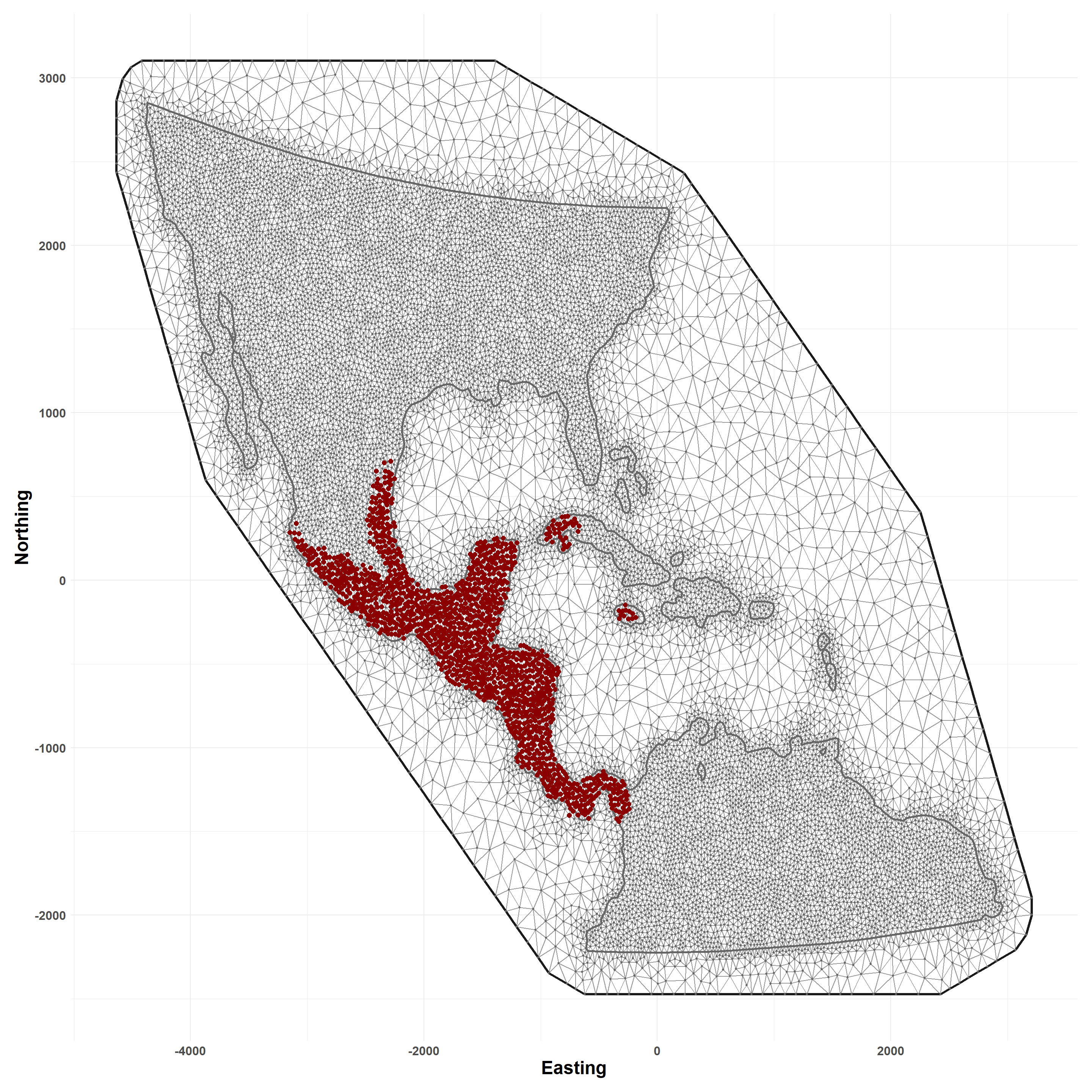
Simulated NWS cases overlain as points.

Show R Code

plot_mesh(mesh.dom)

Figure 1: Triangulated mesh for the study area with simulates NWS case detection overlain.

7 Natural Neighborhoods

Apply tessellation to mesh vertices to identify area of support, or natural neighborhoods around each. Here, this is done using the custom convert_mesh_poly() function.

Show R Code

# mesh areas to polygons
mesh_polys <- convert_mesh_poly(mesh.dom)

# to spatvector and project
mesh_polys <- vect(mesh_polys)
crs(mesh_polys) <- crs(states_proj)

# calculate area
mesh_polys$area <- expanse(mesh_polys, unit = "km")

7.1 Plot Neighborhoods

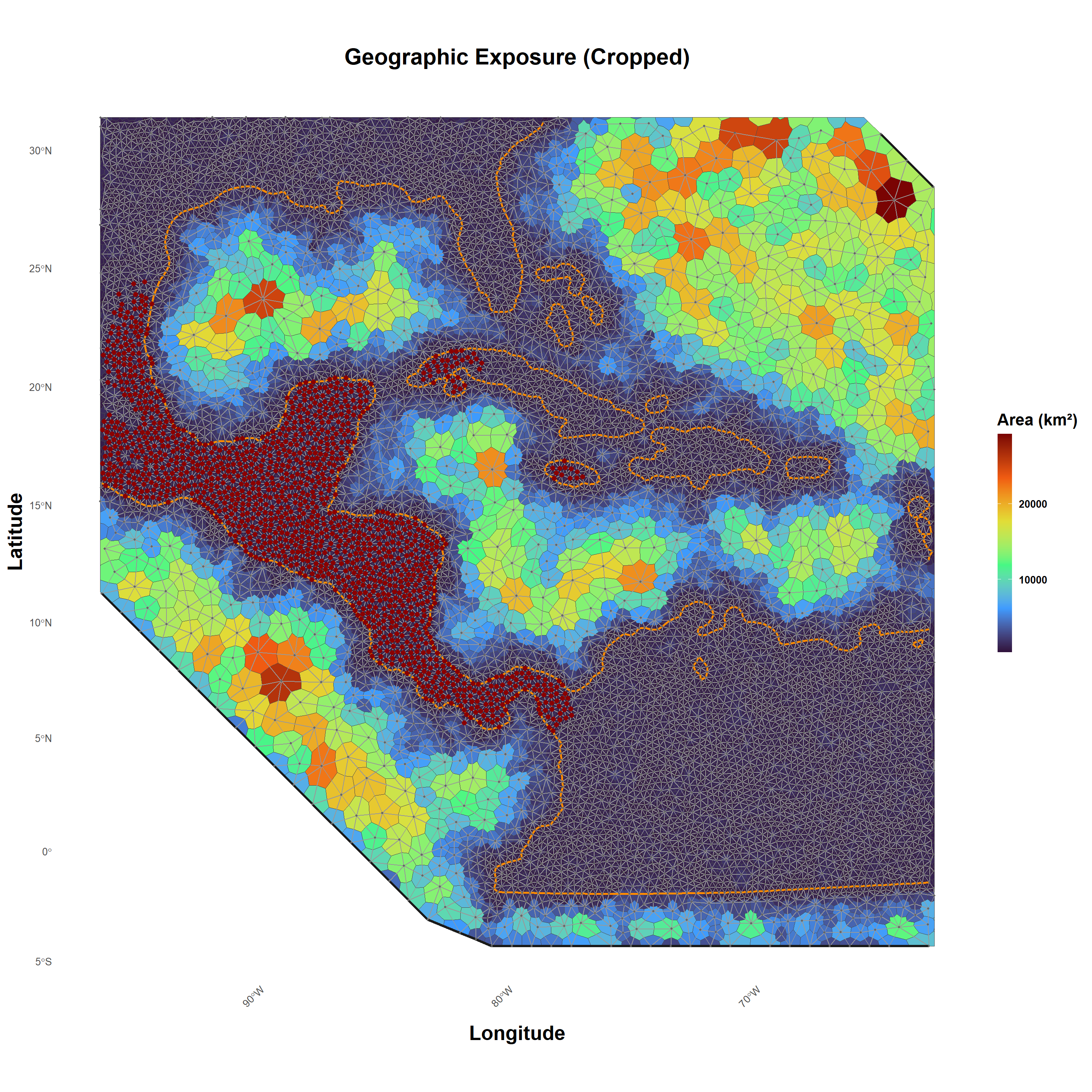
Visual inspection of study area with neighborhoods color coded by geographic area and overlain with mesh and nodes.

Show R Code

mesh_polys_sf <- sf::st_as_sf(mesh_polys)

plot_duel_mesh(mesh_polys_sf, mesh.dom,
               bbox = c(xmin = -2500, # zoom to location extent
                        ymin = -2500, 
                        xmax = 1500, 
                        ymax = 1500))

Figure 2: Tessellation around mesh nodes to identify natural neighborhoods. Zoomed view shows major terrestrial boundaries, mesh, and simulated NWS case detections overlain on neighborhoods. Neighborhoods are colored by geographic area.

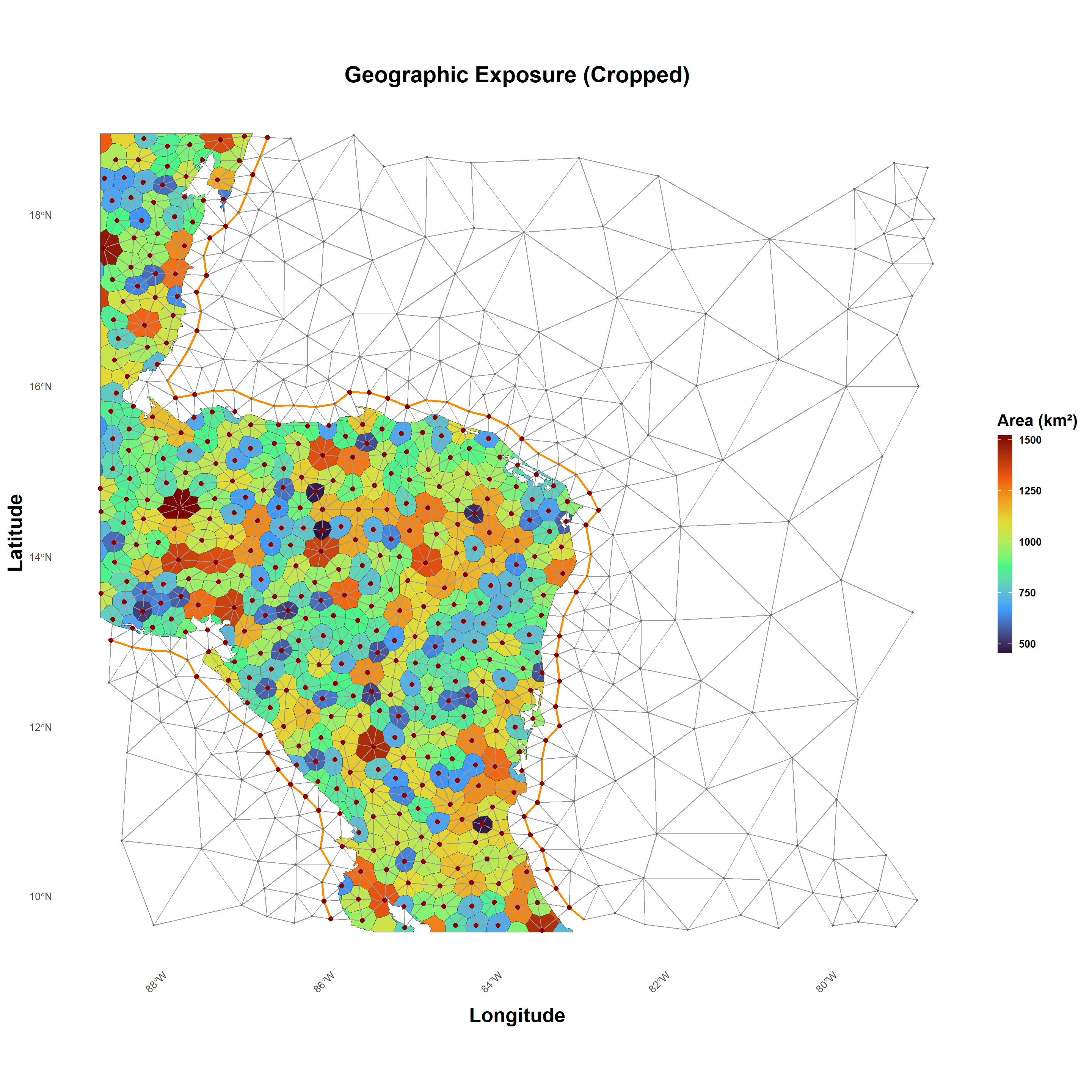
Zoom in closer and remove ocean neighborhoods to improve visualization.

Show R Code

states_simple_sf <- st_as_sf(states_simple)
mesh_polys_sf_crop <- st_intersection(mesh_polys_sf, states_simple_sf)

plot_duel_mesh(mesh_polys_sf_crop, mesh.dom,
               bbox = c(xmin = -1500, # zoom location
                        ymin = -1100, 
                        xmax = -400, 
                        ymax = -50))

Figure 3: Tessellation around mesh nodes to identify natural neighborhoods. Zoomed view shows mesh and simulated NWS case detections overlain on neighborhoods. Neighborhoods are colored by geographic area, with those over major waterbodies have been removed for clarity.

7.2 Save Mesh and Tesselation

Save the triangulated mesh and areal tessellation for the next step.

Show R Code

# save mesh
saveRDS(mesh.dom, here("demo/mesh.rds"))

# copy of natural neighborhoods
writeVector(mesh_polys, here("demo/neighboorhoods.gpkg"), overwrite = TRUE)

Next Step

Once the triangulated mesh and natural neighborhoods have been created and saved, proceed to proceed to the Response page of this site.