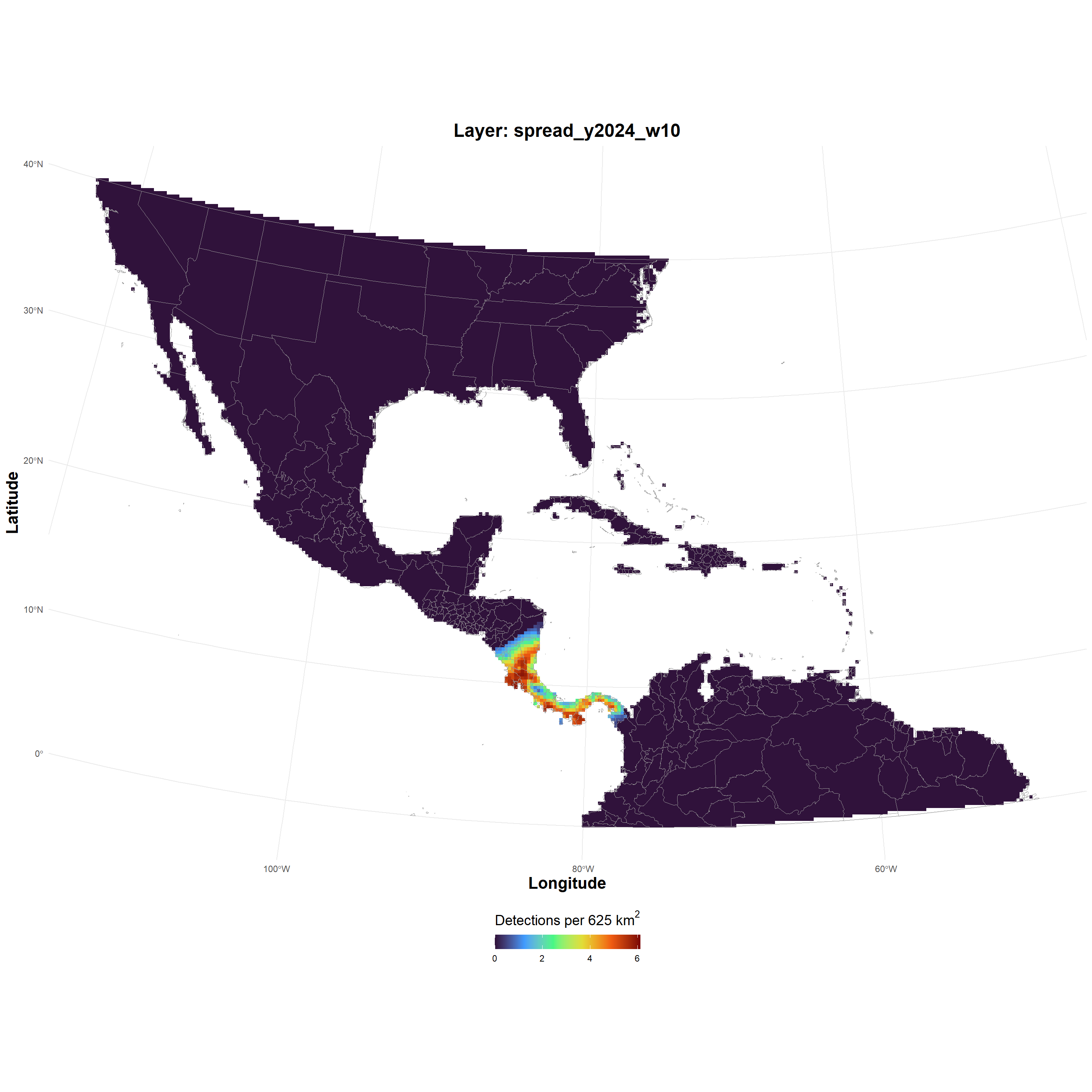
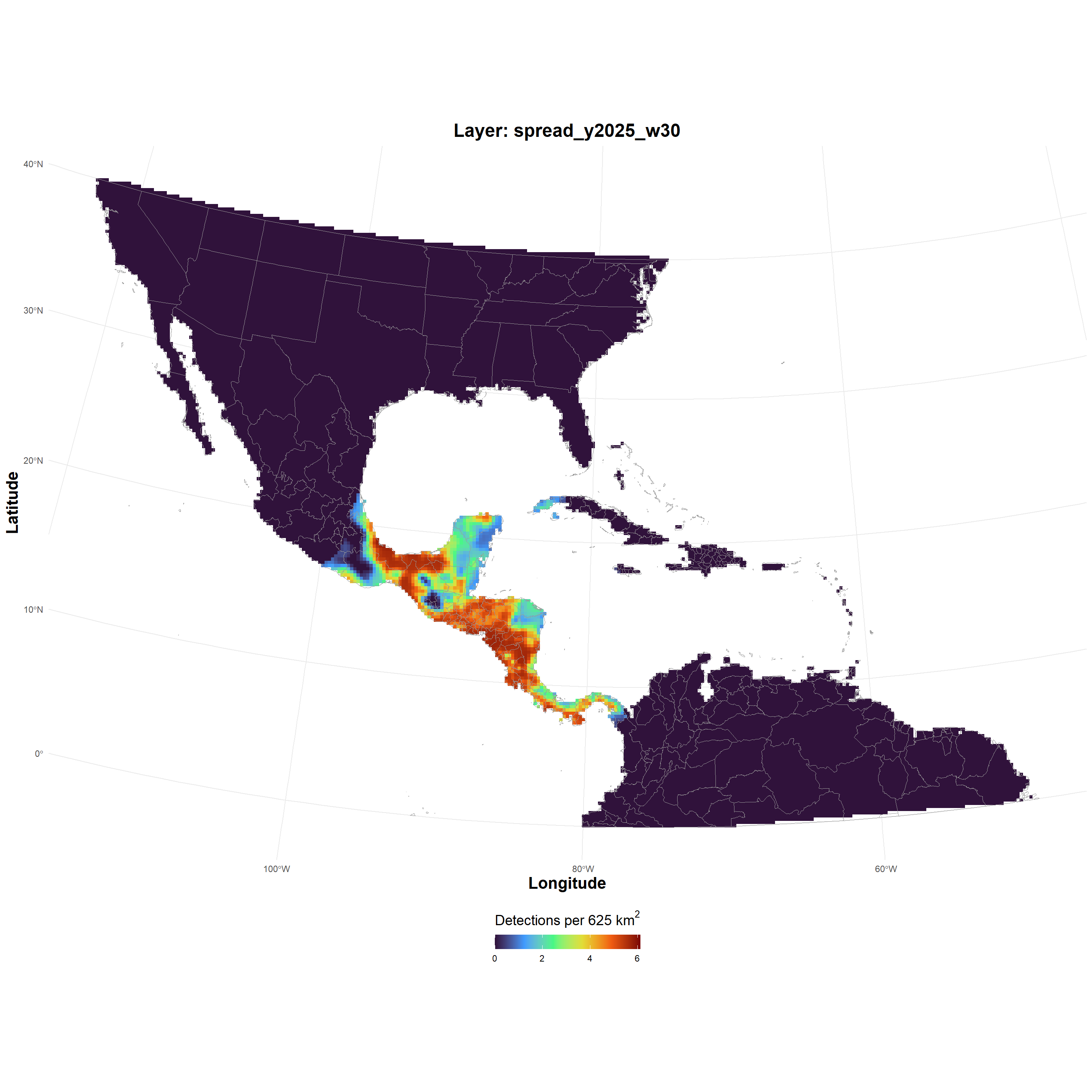
| spread_GeoTIFF_2026-03-24.zip |
69c2d3a4e03dca33dc229717 |
demo/spread_GeoTIFF_2026-03-24.zip |
spread_GeoTIFF_2026-03-24.zip , file , /69c2d3a4e03dca33dc229717 , 2465016 , osfstorage , /spread_GeoTIFF_2026-03-24.zip , 1774375844 , 1774375844 , 09634b49a5a4cf7152e86cceaee889e0 , d1b3407a37034b84c5e5e62dd39fce63f265b92ec42b0f7e8d1e4119aee1546c , 10 , FALSE , 1 , FALSE , https://api.osf.io/v2/files/69c2d3a4e03dca33dc229717/ , https://files.osf.io/v1/resources/uvqmw/providers/osfstorage/69c2d3a4e03dca33dc229717 , https://files.osf.io/v1/resources/uvqmw/providers/osfstorage/69c2d3a4e03dca33dc229717 , https://files.osf.io/v1/resources/uvqmw/providers/osfstorage/69c2d3a4e03dca33dc229717 , https://osf.io/download/69c2d3a4e03dca33dc229717/ , https://mfr.osf.io/render?url=https%3A%2F%2Fosf.io%2Fdownload%2F69c2d3a4e03dca33dc229717%2F%3Fdirect%26mode%3Drender, https://osf.io/uvqmw/files/osfstorage/69c2d3a4e03dca33dc229717 , https://api.osf.io/v2/files/69c2d3a4e03dca33dc229717/ , https://api.osf.io/v2/files/69c2b365ae03e5ce6d107b09/ , 69c2b365ae03e5ce6d107b09 , files , https://api.osf.io/v2/files/69c2d3a4e03dca33dc229717/versions/ , https://api.osf.io/v2/nodes/uvqmw/ , uvqmw , nodes , https://api.osf.io/v2/nodes/uvqmw/ , nodes , nodes , uvqmw , https://api.osf.io/v2/files/69c2d3a4e03dca33dc229717/cedar_metadata_records/ |
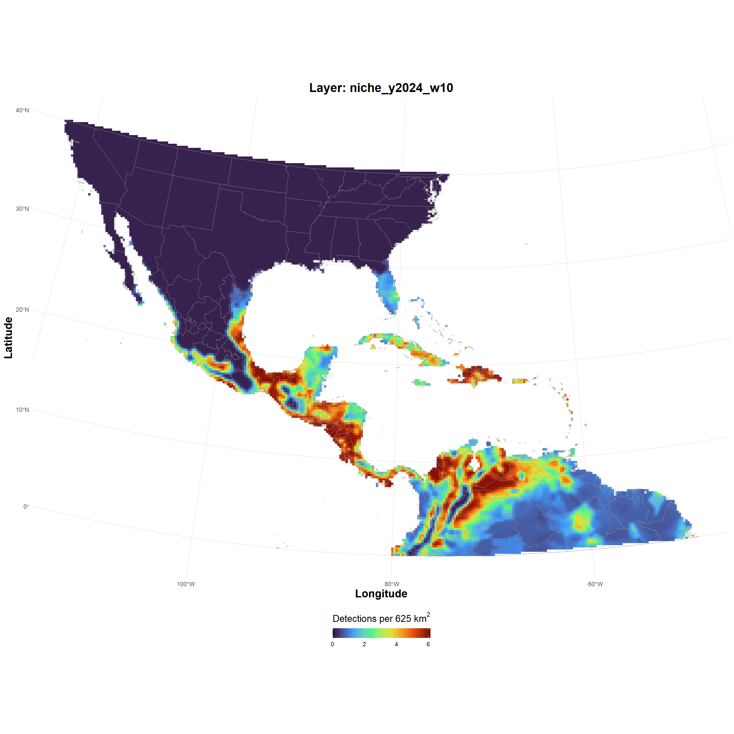
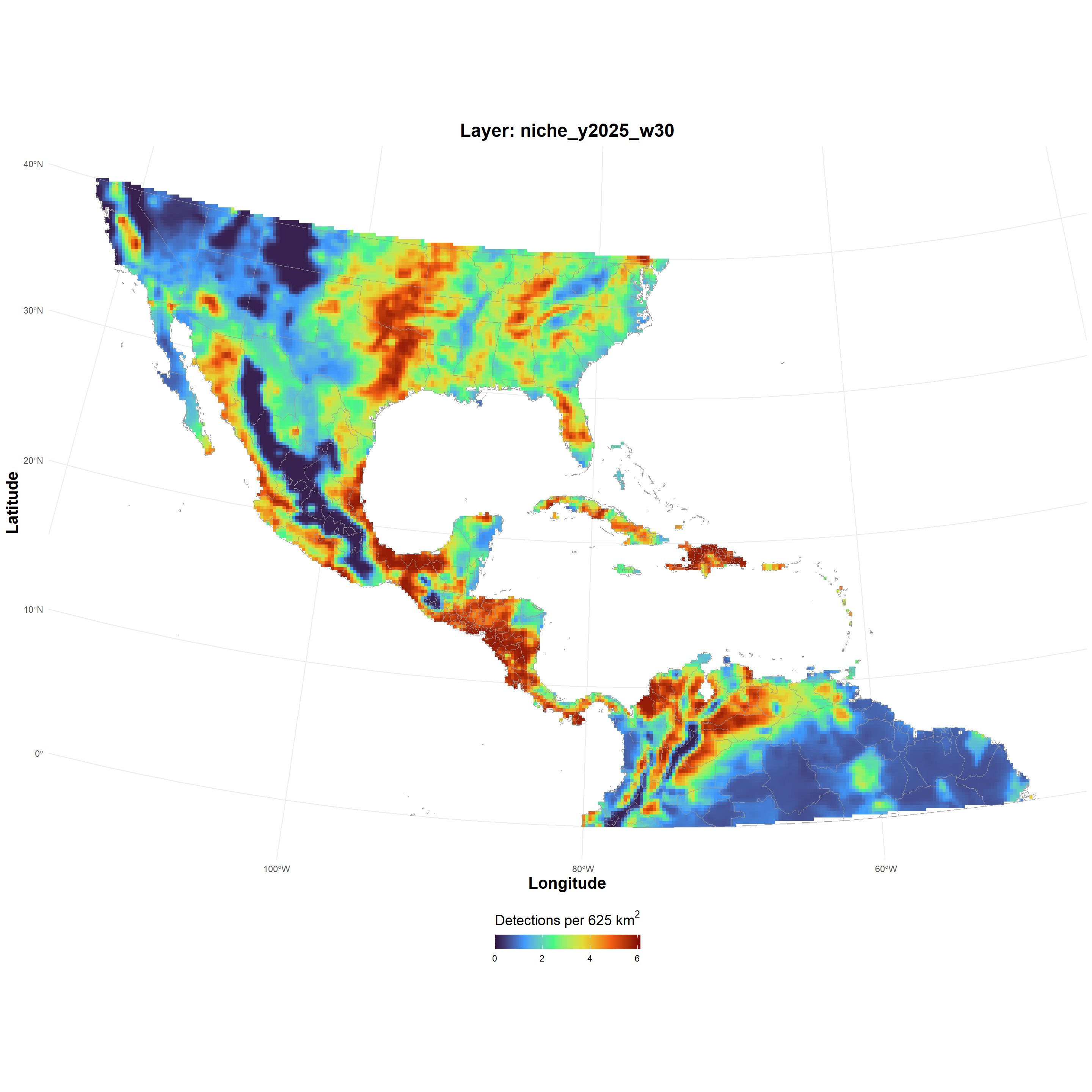
| niche_GeoTIFF_2026-03-24.zip |
69c3204a686690fea0927d64 |
demo/niche_GeoTIFF_2026-03-24.zip |
niche_GeoTIFF_2026-03-24.zip , file , /69c3204a686690fea0927d64 , 12205660 , osfstorage , /niche_GeoTIFF_2026-03-24.zip , 1774395466 , 1774395466 , eb0bbf520ebbb15df84d02ad2222e6c3 , 28dd79fcc7f42242a3e9b1b68ba6598875452d77de9a5453e1bf5e791f76baaa , 9 , FALSE , 1 , FALSE , https://api.osf.io/v2/files/69c3204a686690fea0927d64/ , https://files.osf.io/v1/resources/uvqmw/providers/osfstorage/69c3204a686690fea0927d64 , https://files.osf.io/v1/resources/uvqmw/providers/osfstorage/69c3204a686690fea0927d64 , https://files.osf.io/v1/resources/uvqmw/providers/osfstorage/69c3204a686690fea0927d64 , https://osf.io/download/69c3204a686690fea0927d64/ , https://mfr.osf.io/render?url=https%3A%2F%2Fosf.io%2Fdownload%2F69c3204a686690fea0927d64%2F%3Fdirect%26mode%3Drender, https://osf.io/uvqmw/files/osfstorage/69c3204a686690fea0927d64 , https://api.osf.io/v2/files/69c3204a686690fea0927d64/ , https://api.osf.io/v2/files/69c2b365ae03e5ce6d107b09/ , 69c2b365ae03e5ce6d107b09 , files , https://api.osf.io/v2/files/69c3204a686690fea0927d64/versions/ , https://api.osf.io/v2/nodes/uvqmw/ , uvqmw , nodes , https://api.osf.io/v2/nodes/uvqmw/ , nodes , nodes , uvqmw , https://api.osf.io/v2/files/69c3204a686690fea0927d64/cedar_metadata_records/ |
| study_polygons.gpkg |
69c2c12bcf7cb14d7b48c456 |
demo/study_polygons.gpkg |
study_polygons.gpkg , file , /69c2c12bcf7cb14d7b48c456 , 2670592 , osfstorage , /study_polygons.gpkg , 1774371115 , 1774371115 , 08c72aa055cb38b1473caa3a8063527c , 6734b6f66ebf27962f003e81962bd391cf1381fc74660ddabe64b01fc68b8160 , 11 , FALSE , 1 , FALSE , https://api.osf.io/v2/files/69c2c12bcf7cb14d7b48c456/ , https://files.osf.io/v1/resources/uvqmw/providers/osfstorage/69c2c12bcf7cb14d7b48c456 , https://files.osf.io/v1/resources/uvqmw/providers/osfstorage/69c2c12bcf7cb14d7b48c456 , https://files.osf.io/v1/resources/uvqmw/providers/osfstorage/69c2c12bcf7cb14d7b48c456 , https://osf.io/download/69c2c12bcf7cb14d7b48c456/ , https://mfr.osf.io/render?url=https%3A%2F%2Fosf.io%2Fdownload%2F69c2c12bcf7cb14d7b48c456%2F%3Fdirect%26mode%3Drender, https://osf.io/uvqmw/files/osfstorage/69c2c12bcf7cb14d7b48c456 , https://api.osf.io/v2/files/69c2c12bcf7cb14d7b48c456/ , https://api.osf.io/v2/files/69c2b365ae03e5ce6d107b09/ , 69c2b365ae03e5ce6d107b09 , files , https://api.osf.io/v2/files/69c2c12bcf7cb14d7b48c456/versions/ , https://api.osf.io/v2/nodes/uvqmw/ , uvqmw , nodes , https://api.osf.io/v2/nodes/uvqmw/ , nodes , nodes , uvqmw , https://api.osf.io/v2/files/69c2c12bcf7cb14d7b48c456/cedar_metadata_records/ |
| sim_locations_2026-03-24.csv |
69c2f06142e811a7159282bc |
demo/sim_locations_2026-03-24.csv |
sim_locations_2026-03-24.csv , file , /69c2f06142e811a7159282bc , 17625680 , osfstorage , /sim_locations_2026-03-24.csv , 1774383201 , 1774383201 , 90d4cf68473c797fb0d4b8b007fa9519 , 852f7fc148ea5051bc70337ac34ad51f5f8c59f536d88a6f2a555ab8c9cf956d , 9 , FALSE , 1 , FALSE , https://api.osf.io/v2/files/69c2f06142e811a7159282bc/ , https://files.osf.io/v1/resources/uvqmw/providers/osfstorage/69c2f06142e811a7159282bc , https://files.osf.io/v1/resources/uvqmw/providers/osfstorage/69c2f06142e811a7159282bc , https://files.osf.io/v1/resources/uvqmw/providers/osfstorage/69c2f06142e811a7159282bc , https://osf.io/download/69c2f06142e811a7159282bc/ , https://mfr.osf.io/render?url=https%3A%2F%2Fosf.io%2Fdownload%2F69c2f06142e811a7159282bc%2F%3Fdirect%26mode%3Drender, https://osf.io/uvqmw/files/osfstorage/69c2f06142e811a7159282bc , https://api.osf.io/v2/files/69c2f06142e811a7159282bc/ , https://api.osf.io/v2/files/69c2b365ae03e5ce6d107b09/ , 69c2b365ae03e5ce6d107b09 , files , https://api.osf.io/v2/files/69c2f06142e811a7159282bc/versions/ , https://api.osf.io/v2/nodes/uvqmw/ , uvqmw , nodes , https://api.osf.io/v2/nodes/uvqmw/ , nodes , nodes , uvqmw , https://api.osf.io/v2/files/69c2f06142e811a7159282bc/cedar_metadata_records/ |