The script demonstrates how to expand and index reported NWS case detections and mesh nodes to ensure that all weeks are represented in the data set. Additionally, the script shows how to aggregate individual detection counts to natural natural neighborhoods as needed for the abundance tier in the joint model described in the associated paper.
Once data has been formatted correctly, it can be organized as a bivariate response variable such that Tier 1 describes point-level NWS case detections:
y_{1it} =
\begin{cases}
1, & \text{NWS detection reported at location } i \text{ and time } t \\
0, & \text{NWS not detected or reported at location } i \text{ and time } t
\end{cases}
and, Tier 2 represents the number of NWS Cases reported in each neighborhood:
y_{2it} =
\begin{cases}
NA, & \text{NWS detections not reported in neighborhood } i \text{ and time } t \\
\text{Count}, & \text{Sum of all NWS detections in neighboorhood } i \text{ and time } t
\end{cases}
Note
This script assumes that supporting data has already been downloaded to a directory called /demo, that NWS case detections have been simulated as described on the Simulation tab, and that the triangulated mesh and areal tessellation presented on the tessellation tab have been constructed and saved.
2 Libraries
Load needed libraries and packages.
Show R Code
library(tidyverse) # data wranglingoptions(dplyr.summarise.inform =FALSE)library(here) # directory managementlibrary(patchwork)# combine ggplotslibrary(pals) # color paletteslibrary(osfr) # interact with Open Science Framework (OSF, data repository)library(terra) # spatial data manipulationlibrary(sf) # spatial data manipulationlibrary(spatstat) # spatial data manipulationlibrary(raster) # spatial data manipulationselect <- dplyr::select # deconflict dplyr w/raster # see https://www.r-inla.org/home# install.packages("INLA",repos=c(getOption("repos"),INLA="https://inla.r-inla-download.org/R/stable"), dep=TRUE)library(INLA) # mesh construction, inference
# simulated case detectionssim_data_df <-read_csv(here("demo/sim_locations_demo.csv"))# triangulated meshmesh.dom <-readRDS(here("demo/mesh.rds"))# tessellationmesh_polys <-st_read(here("demo/neighboorhoods.gpkg"))
Reading layer `neighboorhoods' from data source
  `D:\Github\hominivorax-geostat\demo\neighboorhoods.gpkg' using driver `GPKG'
Simple feature collection with 15346 features and 1 field
Geometry type: MULTIPOLYGON
Dimension:     XY
Bounding box:  xmin: -4633.52 ymin: -2473.057 xmax: 3209.094 ymax: 3100.675
Projected CRS: +proj=aea +lat_0=20 +lon_0=-75 +lat_1=10 +lat_2=30 +x_0=0 +y_0=0 +datum=WGS84 +units=km +no_defs
Show R Code
# study area administrative boundariesstates_proj <-st_read(here("demo/study_polygons.gpkg"))
Reading layer `study_states' from data source
  `D:\Github\hominivorax-geostat\demo\study_polygons.gpkg' using driver `GPKG'
Simple feature collection with 492 features and 122 fields
Geometry type: MULTIPOLYGON
Dimension:     XY
Bounding box:  xmin: -4363.574 ymin: -2203.058 xmax: 2962.346 ymax: 2835.693
Projected CRS: +proj=aea +lat_0=20 +lon_0=-75 +lat_1=10 +lat_2=30 +x_0=0 +y_0=0 +datum=WGS84 +units=km +no_defs
Geographic projection of simulated NWS detections (currently unprojected)
Show R Code
sim_data_pnts <-vect(sim_data_df, geom =c("x", "y"), "EPSG:4326") # to pointssim_data_pnts <-project(sim_data_pnts, states_proj) # match other data projection# back to dataframesim_data_df <-as.data.frame(sim_data_pnts, geom ="xy")
5 Prepare Node Locations
Show R Code
# get node coordinatesint_pnts <-as.data.frame(cbind(mesh.dom$loc[,1], mesh.dom$loc[,2]))names(int_pnts) <-c("x", "y")# convert to pointsint_pnts <-vect(int_pnts, geom =c("x", "y"), crs = states_proj)
Identify and remove nodes located in oceans (non-NWS habitat)
Show R Code
states_simple <-vect(states_proj)states_simple$inside <-1int_pnts$inside <-extract(states_simple["inside"], int_pnts)$inside# back to dataframeinteg_df <-as.data.frame(int_pnts, geom="xy") %>%filter(!is.na(inside)) %>%# remove ocean nodesmutate(Y1 =0, # no detectionExp =NA) %>%# no exposure (point locations, no area)select(Y1, Exp, x, y)
6 Time Expansion
Create dataframe with all years and weeks for the study period, weeks between 2022-01-01 and 2026-03-01.
Show R Code
study_start <-as_date("2022-01-01")study_end <-as_date("2026-03-01")data_weeks <- sim_data_df %>%distinct(year, week)# date sequence to fill gaps with no NWScalendar_weeks <-data.frame(date =seq(study_start, study_end, by ="day")) %>%mutate(year =epiyear(date),week =epiweek(date) ) %>%distinct(year, week)time_index <-bind_rows(data_weeks, calendar_weeks) %>%distinct(year, week) %>%mutate(year =as.numeric(year), week =as.numeric(week)) %>%filter(year >=2022) %>%arrange(year, week)
Replicate nodes to ensure a copy for each week in the study period.
# assign unique polygon IDmesh_polys$poly_id <-1:nrow(mesh_polys)# get the polygon ID for each NWS reported detection (or node)tier1_pnts <-vect(tier1_df, geom =c("x", "y"), crs = states_proj) # to spatial pointsmesh_polys <-vect(mesh_polys) # convert to SpatVectorextracted <-extract(mesh_polys, tier1_pnts) # add ID to dataframetier1_df$poly_id <- extracted$poly_id# count points in each polygon by year-weekcounts <- tier1_df %>%filter(Y1 ==1) %>%# only count detections, not nodes (Y1==0)count(poly_id, year, week, name ="n_points")range(counts$n_points) # max simulated detections in neighborhood and week
[1] 1 27
10 Match to Neighborhood
Lastly, aggregate counts per neighborhood are match to the location of that neighborhood centroid.
Show R Code
# get centroid coordinatescentroids <-centroids(mesh_polys)mesh_centroids_df <-as.data.frame(geom(centroids)[, c("x", "y")])mesh_centroids_df$poly_id <- mesh_polys$poly_id# all combinations of poly_id and time# making a copy for each week in the study periodall_combos <- mesh_centroids_df %>%select(poly_id, x, y) %>%crossing(time_index)# match with aggregate counts# fill with NA if no NWS at location of time stepweekly_counts <- all_combos %>%left_join(counts, by =c("poly_id", "year", "week")) %>%arrange(poly_id, year, week)sum(weekly_counts$n_points, na.rm=TRUE) ==sum(counts$n_points) #verify all counts were matched
[1] TRUE
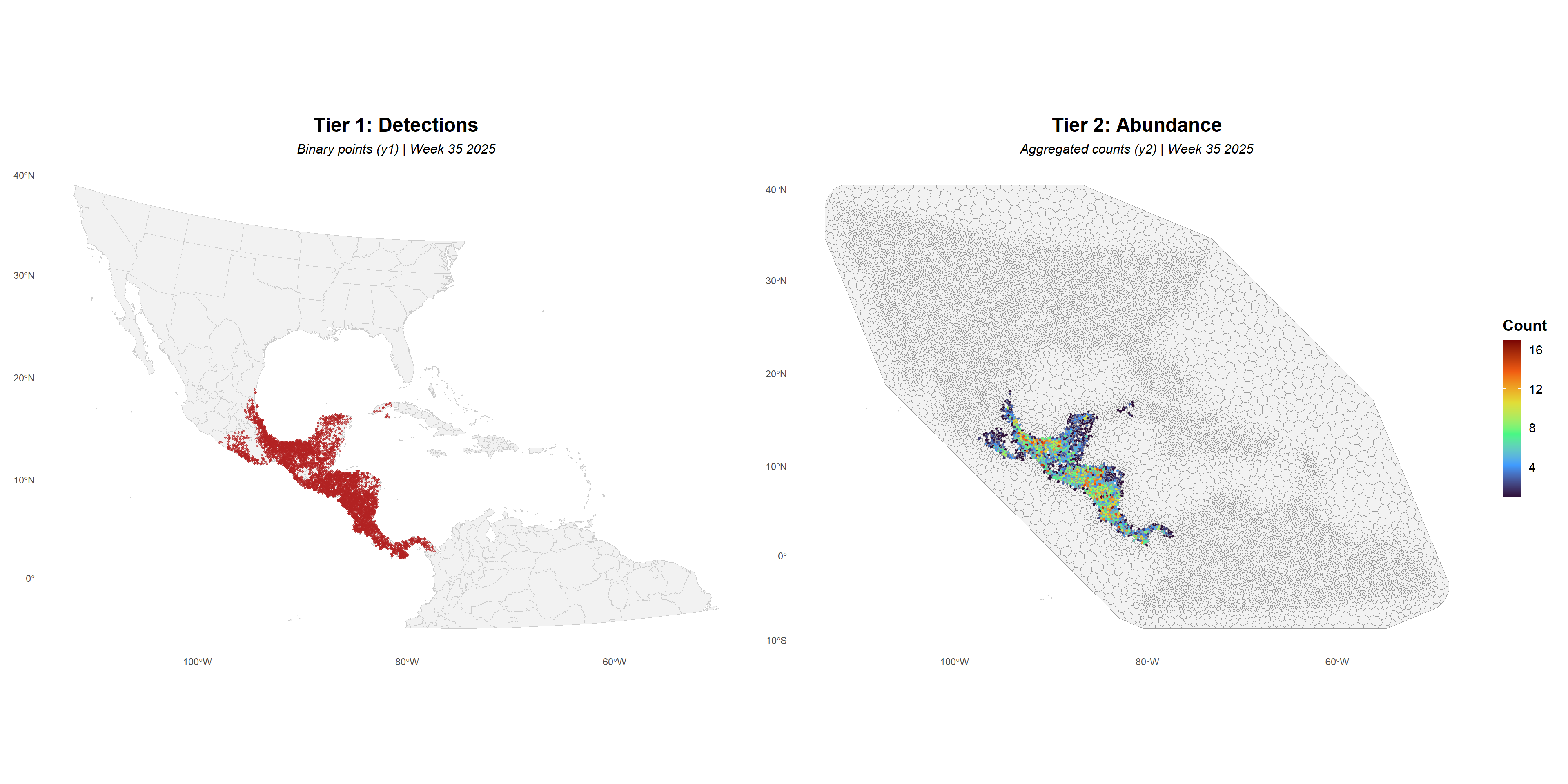
11 Map Response
Viewing the detection and count data for a select year and week.
Show R Code
# convert to SF for plottingtier1_sf <-st_as_sf(tier1_df, coords =c("x", "y"), crs =st_crs(states_proj))tier2_sf <- mesh_polys %>%st_as_sf() %>%inner_join(weekly_counts, by ="poly_id")
Figure 1: Comparison of data used as bivariate response variable for detection (left) and potential abundance (right) tiers for arbitrary week. Panel at left shows point-level location of simulated detections whereas that at right shows sum of detections per neighborhood.
Next Step
Proceed to the next step to view the model specification.