Overview

Supporting Information

This site provides a demonstrative workflow and supporting information for the publication:
Modeling the 2014-2015 Vesicular Stomatitis Outbreak in the United States using an SEIR-SEI Approach

Authors:
Humphreys, Pelzel-McCluskey, Shults, Velazquez Salinas, Bertram, McGregor, Cohnstaedt, Swanson, Scroggs, Fautt, Mooney, Peters, and Rodriguez

Viruses 2024, 16, 1315. https://doi.org/10.3390/v16081315

External Resources

An interactive dashboard to demonstrate the described SEIR-SEI model is available: ShinyApps: https://geoepi.shinyapps.io/seir-vector/

Code for this site and ShinyApp above are available:
GitHub: https://github.com/geoepi/seir-vector

Large model objects, incidence data, and other archived information are available on the Open Science Framework: Project OSF site: https://osf.io/vqgxs/. The R-function get_data_osf() is provided to download and read these data.

Workflow Synopsis

This script provides an overview of the methodologies and code presented in the publication above. Note that data, code, and website configuration files, as well as code for the VSV ShinyApp, are available on the project’s GitHub site and OSF Project site. Executed Stan model objects are approximately 200mb in size, code to download and read these objects is provided in the script.

For simplicity, this workflow will demonstrate analysis for outbreaks observed in 2014, however the workflow can be applied to 2015 outbreaks with minimal modification. The PAGE CONTENTS menu in the right upper corner can be used to navigate to specific sections.

Parameters and Formula

Model Parameters

Brief descriptions of parameters used in the model. Note that additional information and cited sources for selected parameter values are provided in the associated publication.

\begin{array}{|c|l|} \hline \text{Parameter} & \text{Description} \\ \hline N_h & \text{Total number of vertebrate hosts} \\ N_v & \text{Total number of insect vectors} \\ \upsilon_h & \text{Contact rate, bites sustained by host} \\ \upsilon_v & \text{Contact rate, vector biting rate} \\ \beta_h & \text{Vector to host transmission probability} \\ \beta_v & \text{Host to vector transmission probability} \\ \sigma_h & \text{Intrinsic Incubation Period (IIP)} \\ \sigma_v & \text{Extrinsic Incubation Period (EIP)} \\ \gamma_h & \text{Host removal rate (recovery or quarantine)} \\ \rho_h & \text{Host heterogeneous competency} \\ \rho_v & \text{Vector heterogeneous competency} \\ \mu_v & \text{Vector background mortality rate} \\ \kappa & \text{Observation bias (proportion observed)} \\ \hline \end{array}

Model Specification

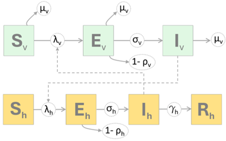
Mechanistic aspects of the model can can be diagrammatically represented as shown below. Note that in case of both the vertebrate hosts (h subscript) and vectors (v subscript), the term \rho influences the number of exposed individuals (E) that proceed to the infectiousness compartment (I).

More formally, the model is given as:

\begin{align} \lambda_h &= \upsilon_h \cdot \beta_h \cdot \frac{I_v}{N_v} \\ \lambda_v &= \upsilon_v \cdot \beta_v \cdot \frac{I_h}{N_h} \\ \frac{dS_h}{dt} &= -\lambda_h \cdot S_h \\ \frac{dE_h}{dt} &= \lambda_h \cdot S_h - \sigma_h \cdot E_h \\ \frac{dI_h}{dt} &= \sigma_h \cdot E_h \cdot \rho_h - \gamma_h \cdot I_h \\ \frac{dR_h}{dt} &= \gamma_h \cdot I_h \\ \frac{dS_v}{dt} &= \mu_v \cdot N_v - \lambda_v \cdot S_v - \mu_v \cdot S_v \\ \frac{dE_v}{dt} &= \lambda_v \cdot S_v - (\sigma_v + \mu_v) \cdot E_v \\ \frac{dI_v}{dt} &= \sigma_v \cdot E_v \cdot \rho_v - \mu_v \cdot I_v \\ \nonumber \end{align} \tag{1}

in which the first two lines give the Force of Infection (FOI, \lambda’s) for hosts and vectors respectively and \rho parameters (range 0.00-1.00) potentially reduce the size of the exposed (E) populations used in calculating the number of infectious individuals (I).

Model Preliminaries

Before constructing a Bayesian model in Stan (Stan Installation), we first visualize the data and construct an exploratory compartmental model using non-Bayesian Ordinary Differential Equations (ODE) and the deSolve Package.

Needed Libraries

Load needed R-Packages and custom functions.

Hide code

library(here) # to manage directories
library(tidyverse) # data wrangling
library(deSolve) # for exploratory models
library(ggdist) # visualizations
library(rstan) # interface with Stan from R
rstan_options(auto_write = TRUE) # options
options(mc.cores = parallel::detectCores())

library(cmdstanr) # additional Stan options in R
check_cmdstan_toolchain(fix = TRUE, quiet = TRUE)
register_knitr_engine()

# custom functions (mostly plotting)  
source(here("./R/utilities.R"))
source_dir("./R")

Observed Incidence

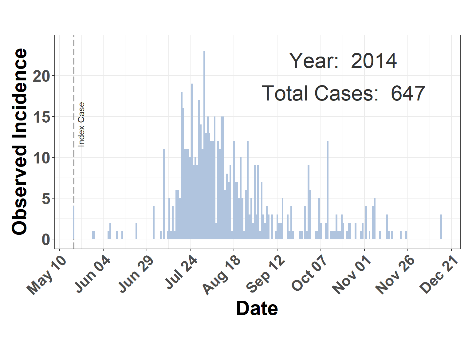
Read observed incidence data as a data frame called truth_df and create a simple plot figure. Note that 2014 and 2015 data are available in the vsv_ind_truth.rds object.

Contents for truth_df

• date: Estimated date of disease onset (symptoms) as determined by examination at time of inspection.
  
• count: Number of individuals animals with Vesicular Stomatitis (VS)
  
• susc: Number of individual animals located with same herd or on same premises as confirmed animal. These values are assumed to reflect susceptible animals.
  
• year: Year of confirmed VS onset.
  
• doy: Integer 1-365 reflecting the day of year for the date.

Hide code

truth_df <- get_data_osf("vs_inc_truth") |>
  filter(year == 2014) # change to 2015 to examine 2015 data

File downloaded successfully and saved as vs_inc_truth.rds 

Hide code

str(truth_df)

'data.frame':   117 obs. of  5 variables:
 $ date : Date, format: "2014-05-18" "2014-05-29" ...
 $ count: int  4 1 1 1 2 1 1 2 4 1 ...
 $ susc : int  65 3 3 5 4 1 11 79 7 6 ...
 $ year : num  2014 2014 2014 2014 2014 ...
 $ doy  : num  138 149 150 158 159 163 166 174 184 188 ...

Hide code

plot_incidence(truth_df)

Figure 1: Observed VS incidence 2014.

Exploratory Model

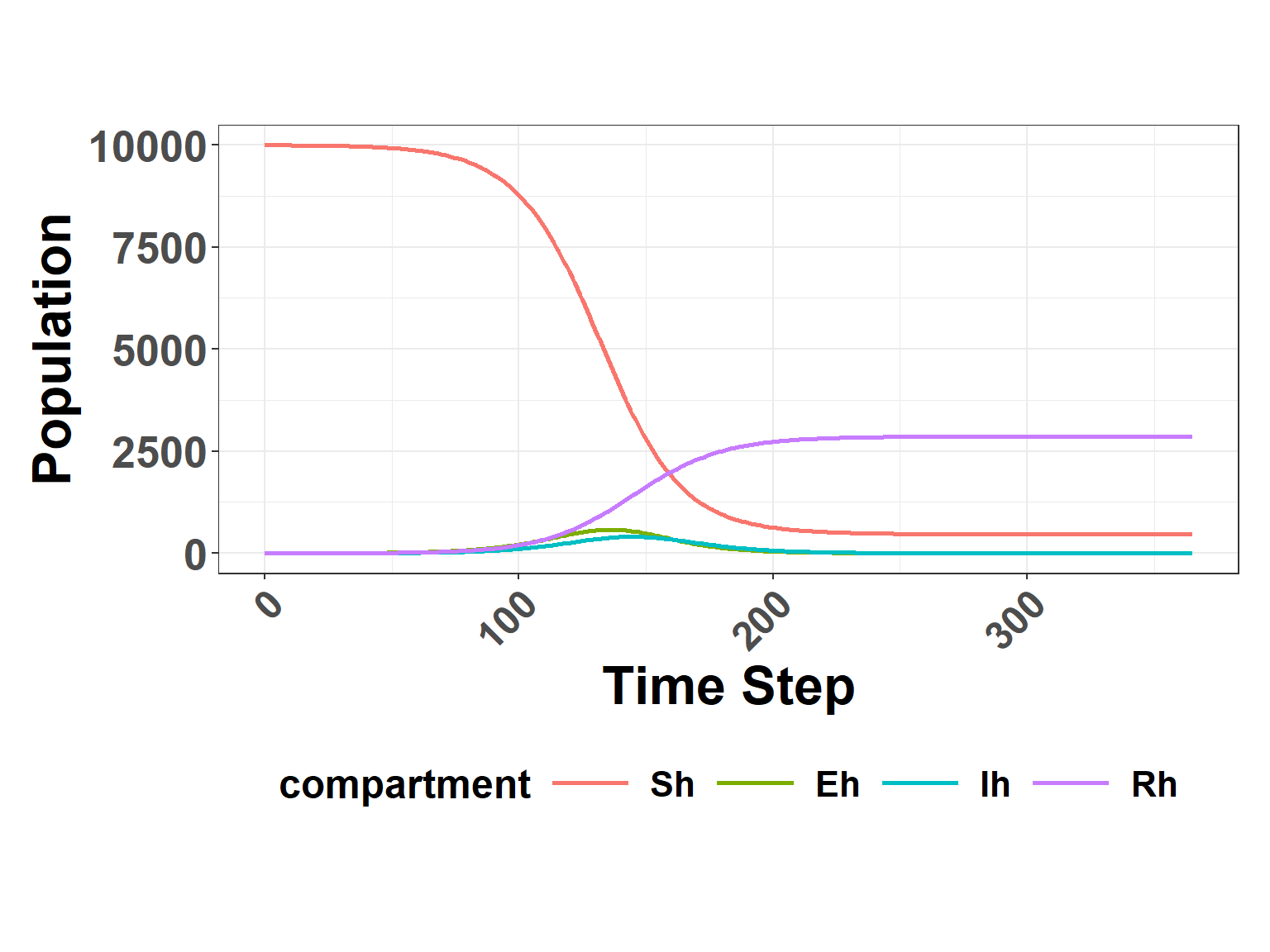
Before coding a Stan model, model parameters are through construction of a relatively simple Ordinary Differential Equations (ODE) model using the deSolve package. This model uses discrete, user specified values and does not incorporate uncertainty.

Initial Parameters

Parameters are describe in the Table at top of page. The specific values given in this example were arbitrarily selected from the ranges evaluated in the full model (presented later in script).

Hide code

initial_parameters <- c(
  beta_h = 0.95,
  gamma_h = 0.10,
  sigma_h = 0.25,
  sigma_v = 0.4,
  rho_h = 0.3,
  rho_v = 0.85,
  beta_v = 0.85,
  mu_v = 0.1,
  upsilon_h = 0.6,
  upsilon_v = 0.35
)

Initial Conditions

Initial population estimates and counts of exposed and infectious individuals.

Hide code

N_h <- 10000   # number of vertebrate hosts
Eh <- 0        # initial hosts exposed
Ih <- 1        # initial hosts infectious
N_v <- 300 * N_h  # number of vectors per host
Ev <- 0        # initial exposed vectors
Iv <- 1        # initial infectious vectors

initial_conditions <- c(
  Sh = N_h - Eh - Ih,  # Susceptible hosts
  Eh = Eh,             # Exposed hosts
  Ih = Ih,             # Infectious hosts
  Rh = 0,              # Recovered hosts
  Sv = N_v - Iv - Ev,  # Susceptible vectors
  Ev = Ev,             # Exposed vectors
  Iv = Iv              # Infectious vectors
)

ODE Function

Results from this exploratory model can be examined more thoroughly on the SEIR-SEI ShinyApp, which uses the same underlying function as given here.

Hide code

seirsei_ode <- function(t, state, parameters) {
  with(as.list(c(state, parameters)), {
    
    lambda_h = upsilon_h * beta_h * Iv / N_v
    lambda_v = upsilon_v * beta_v * Ih / N_h
    
    dSh = -lambda_h * Sh
    dEh = lambda_h * Sh - sigma_h * Eh
    dIh = sigma_h * Eh*rho_h - gamma_h * Ih
    dRh = gamma_h * Ih
    dSv = mu_v * N_v - lambda_v * Sv - mu_v * Sv
    dEv = lambda_v * Sv - (sigma_v + mu_v) * Ev
    dIv = sigma_v * Ev*rho_v - mu_v * Iv
    
    return(list(c(dSh, dEh, dIh, dRh, dSv, dEv, dIv)))
  })
}

Time Steps

Hide code

times <- seq(0, 365, by = 1)

Run Model

Hide code

out <- as.data.frame(
  ode(y = initial_conditions, times = times, func = seirsei_ode, parms = initial_parameters)
)

Plot Results

Hide code

plot_ode_dynamics(out)

Figure 2: Host population dynamics from exploratory model.

Hide code

compare_ei_incidence(out, gamma_h=initial_parameters["gamma_h"])

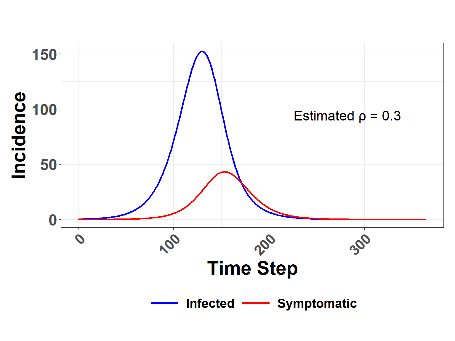
Figure 3: Comparison of incident infections. Line labeled Infected indicates the number of new indiduals added to the Exposed compartment per time step, whereas the line labeled Symptomatic refers to the number of new individuals added to the infectious compartment. The ratio of the sums for the Infected and Symptomatic curves is shown as Estimated rho in the plot. This reverse calculation demonstrates what the rho competency parameter is doing in the model.

Bayesian Model

Having demonstrated model parameter relationships using the ODE function above, a full Bayesian model is next constructed in Stan. The Bayesian approach allows for parameters to specified based on what is currently understood about VSV hosts, vectors, and epidemiology. This done through prior distribution specifications. The Bayesian approach also provides for better accounting of uncertainty in the model.

In addition to translating the SEIR-SEI equations (Equation 1) to the Stan language, a likelihood function is needed as well as incorporation of an additional observation error term to help account for the difference between disease cases as observed and documented and the case number (theoretically) needed to propagate the disease, assuming the model’s mechanistic parameters accurately reflect the reality of the VS epidemiology.

Prior Model

Before incorporating observed data into the model, a prior model is coded and evaluated to ensure that assumptions about prior distributions are reasonable.

Prior model code

functions {
    // SEIR-SEI function
  real[] seirsei(real t, real[] y, real[] theta, 
             real[] x_r, int[] x_i) {

      real N_h = x_i[1];        // parameters are described in table above
      real beta_h = theta[1];
      real gamma_h = theta[2];
      real sigma_h = theta[3];
      real sigma_v = theta[4];
      real rho_h = theta[5];
      real rho_v = theta[6];
      real beta_v = theta[7];
      real mu_v = theta[8];
      real upsilon_h = theta[9];
      real upsilon_v = theta[10];
      real i_0 = theta[11];     // initial conditions
      real e_0 = theta[12];
      real ev_0 = theta[13];
      real iv_0 = theta[14];
      real N_v = theta[15];
      
      // initial compartment sizes
      real init[7] = {N_h - i_0 - e_0, e_0, i_0, 0, N_v - iv_0 - ev_0, ev_0, iv_0}; 
      
      real Sh = y[1] + init[1]; // compartments
      real Eh = y[2] + init[2];
      real Ih = y[3] + init[3];
      real Rh = y[4] + init[4];
      real Sv = y[5] + init[5];
      real Ev = y[6] + init[6];
      real Iv = y[7] + init[7];
      
      // FORCE of Infection
      real lambda_h = upsilon_h * beta_h * Iv / N_v;
      real lambda_v = upsilon_v * beta_v * Ih / N_h;
      
      // differential equations
      real dS_dt = -lambda_h * Sh;
      real dE_dt =  lambda_h * Sh - sigma_h * Eh;
      real dI_dt = sigma_h * Eh*rho_h - gamma_h * Ih;
      real dR_dt =  gamma_h * Ih;
      
      real dSv_dt = mu_v*N_v - lambda_v*Sv - mu_v*Sv;
      real dEv_dt = lambda_v*Sv - (sigma_v + mu_v)*Ev;
      real dIv_dt =  sigma_v * Ev*rho_v - mu_v*Iv;
     
      return {dS_dt, dE_dt, dI_dt, dR_dt, dSv_dt, dEv_dt, dIv_dt};
  }
}
data {
  int<lower=1> n_days; // number of days
  real t0;            // initial step
  real ts[n_days];    // time steps
  int N_h;            // host population size
  int N_v;            // vector population size
}
transformed data {
  real x_r[0];        // data array
  int x_i[1] = { N_h };   // array with host population size
}
parameters {
  real<lower=0, upper=1> beta_h; // parameters, see table above
  real<lower=0> gamma_h;
  real<lower=0> sigma_h;
  real<lower=0> sigma_v;
  real<lower=0, upper=1> rho_h;
  real<lower=0, upper=1> rho_v;
  real<lower=0, upper=1> beta_v;
  real<lower=0> mu_v;
  real<lower=0> upsilon_h;
  real<lower=0> upsilon_v;
  real<lower=0> phi_inv;
  real<lower=0> i_0; 
  real<lower=0> e_0; 
  real<lower=0> ev_0; 
  real<lower=0> iv_0; 
}
transformed parameters{
  real y[n_days, 7];        // outputs, state variables
  real incidence[n_days - 1];   // incidence 
  real phi = 1. / phi_inv;    // dispersian parameter for NegBinomial
  real theta[15] = {beta_h, gamma_h, sigma_h, sigma_v, rho_h, rho_v, beta_v, mu_v, upsilon_h, upsilon_v, i_0, e_0, ev_0, iv_0, N_v};
  
  // solve ODEs using Runge-Kutta 45 integration
  y = integrate_ode_rk45(seirsei, rep_array(0.0, 7), t0, ts, theta, x_r, x_i);
  
  // daily incidence
  for (i in 1:n_days-1){
    incidence[i] = -(y[i+1, 2] - y[i, 2] + y[i+1, 1] - y[i, 1]) + 1e-8;
  }
}
model { // model priors
  beta_h ~ beta(10, 2);
  gamma_h ~ lognormal(log(0.13), 0.1);  
  sigma_h ~ lognormal(log(0.12), 0.1);
  sigma_v ~ lognormal(log(0.4), 0.1);
  rho_h ~ beta(5, 10);
  rho_v ~ beta(10, 2); 
  beta_v ~ beta(10, 2);
  mu_v ~ lognormal(log(0.1), 0.1);
  upsilon_h ~ lognormal(log(0.6), 0.1);
  upsilon_v ~ lognormal(log(0.3), 0.1);
  phi_inv ~ exponential(2);
  i_0 ~ lognormal(0, 0.1);
  e_0 ~ lognormal(0, 0.1);
  ev_0 ~ lognormal(0, 0.1);
  iv_0 ~ lognormal(0, 0.1);
}
generated quantities {
  real duration = 1 / gamma_h; // disease duration
  real incub_h = 1 / sigma_h;   // intrinsic incubation period
  real incub_v = 1/ sigma_v;    // extrinsic incubation period
  real pred_infected[n_days-1];  // predicted incidence
  pred_infected = neg_binomial_2_rng(incidence, phi); // sample from NegBinomial
}

NegativeBinomial Sampling

Note that the Stan code above includes a negative binomial distribution that samples from estimated incidence. The SEIR-SEI ODE equations estimate prevalence but not incidence. Therefore, the code first estimates incidence (new infections each day) using the susceptible (S) and exposed (E) compartments. A small value (1e-8) is included to prevent incidence from being negative on the initial iteration. The code as shown in the transformed parameters block is,

for (i in 1:n_days-1){
    incidence[i] = -(y[i+1, 2] - y[i, 2] + y[i+1, 1] - y[i, 1]) + 1e-8;
  }

Later in the generated quantities block, incidence is used in sampling from the NgBinomial,

real pred_infected[n_days-1]; 
  pred_infected = neg_binomial_2_rng(incidence, phi); 

Consdering that incidence is estimated from the daily change (\Delta \text{I}_{t}) in infections (virus exposures), and this quantity is used to sample from the NegBinomial, the notation with prior distributions couldbe shown as,

\begin{align} \nonumber \text{Y}_{t}|\theta &\sim \text{NegBinomial}(\text{Y}|\Delta\text{I}_{t}, \phi) \\ \nonumber \theta &= \{\upsilon_h,\upsilon_v, \beta_h, \beta_v, \sigma_h, \sigma_v, \gamma_h, \mu, \rho \} \\ \nonumber \upsilon_h &\sim \text{Lognormal}(log(0.25), 0.1) \\ \nonumber \upsilon_v &\sim \text{Lognormal}(log(0.15), 0.1) \\ \nonumber \beta_h &\sim \text{Beta}(10, 1) \\ \nonumber \beta_v &\sim \text{Beta}(1, 10) \\ \sigma_h &\sim \text{Lognormal}(log(0.15), 0.1) \\ \nonumber \sigma_v &\sim \text{Lognormal}(log(0.3), 0.1) \\ \nonumber \rho_h &\sim \text{Beta}(10, 100) \\ \nonumber \rho_v &\sim \text{Beta}(5, 10) \\ \nonumber \gamma_h &\sim \text{Lognormal}(log(0.085), 0.1) \\ \nonumber \mu &\sim \text{Lognormal}(log(0.1), 0.1) \\ \nonumber {1}/{\phi} &\sim \text{Exponential}(2) \\ \nonumber \end{align} \tag{2}

Prior model setup

Organize data needed to run the prior model.

Hide code

# total host population
N = 14160

# time steps 
n_days = 365 
t = seq(0, n_days, by = 1)
t0 = 0 
t = t[-1]

# orgainize data for Stan 
data_seir = list(n_days = n_days, 
                 t0 = t0, 
                 ts = t, 
                 N_h = N, 
                 N_v = 300*N)

str(data_seir)

List of 5
 $ n_days: num 365
 $ t0    : num 0
 $ ts    : num [1:365] 1 2 3 4 5 6 7 8 9 10 ...
 $ N_h   : num 14160
 $ N_v   : num 4248000

Hide code

# number of MCMC steps
niter = 2000

# number of chains, only a short run for prior model
num_chains <- 2

# unique initial values for each chain
init_list <- vector("list", num_chains)

for (i in 1:num_chains) {
  
  init_list[[i]] <- list(beta_h = rbeta(1, 10, 1),
                         gamma_h = rlnorm(1, log(0.15), 0.1),
                         sigma_h = rlnorm(1, log(0.17), 0.1),                         
                         sigma_v = rlnorm(1, log(0.3), 0.1),
                         beta_v = rbeta(1, 15, 100),
                         mu_v = rlnorm(1, log(0.1), 0.1),
                         upsilon_h = rlnorm(1, log(0.25), 0.1),
                         upsilon_v = rlnorm(1, log(0.15), 0.1),   
                         i_0 = runif(1, 1, 2),
                         e_0 = runif(1, 1, 2),
                         ev_0 = runif(1, 1, 2),
                         iv_0 = runif(1, 1, 2))
}

Read stan model

The Stan code above is saved as a text file. It is read in to memory.

Hide code

seirsei.st = stan_model("inst/stan/vsv_prior.stan")

Run prior model

Data, model code, initial values are run. This model has been verified to run, however to reduce run time, a saved copy is loaded below.

Hide code

prior_model <- sampling(seirsei.st,
                        data = data_seir,
                        iter = niter,
                        chains = num_chains,
                        cores = parallel::detectCores(),
                        warmup = 500,
                        save_warmup = FALSE,
                        init = init_list, 
                        seed = 1976) 

load saved model

Hide code

prior_model <- get_data_osf("prior_model")

File downloaded successfully and saved as prior_model.rds 

Hide code

class(prior_model)

[1] "stanfit"
attr(,"package")
[1] "rstan"

Check results

Parameter Distributions
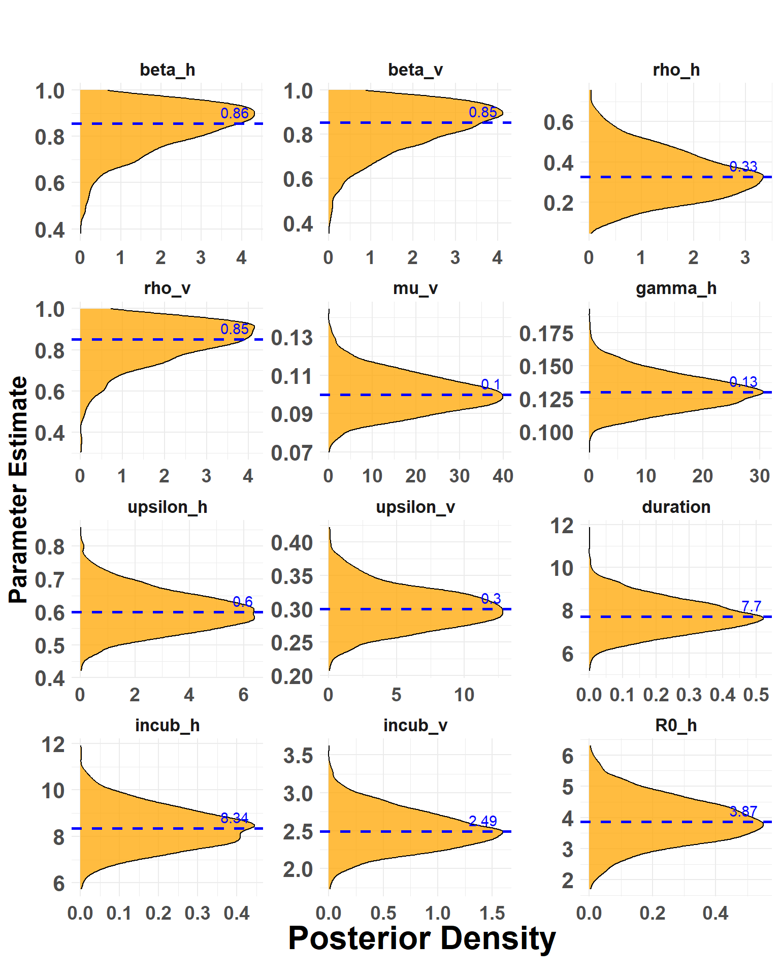
Parameter distributions are plotted with medians as a visual check. In addition to parameters specified in prior distributions, the Extrinsic Incubation Period (incub_v), Intrinsic Incubation Period (incub_h), and basic reproduction number (R0_h) are shown in Figure 4. The EIP and IIP are respectively calculated as the reciprocal of the estimated \sigma_v and \sigma_h parameters. The reproduction number (R_0) is calculated as \beta_h \cdot \upsilon_h/\gamma_h.

Hide code

plot_params_posteriors(prior_model)

No id variables; using all as measure variables

Figure 4: Distributions from modeled priors. Dashed lines show the median value for each parameter.

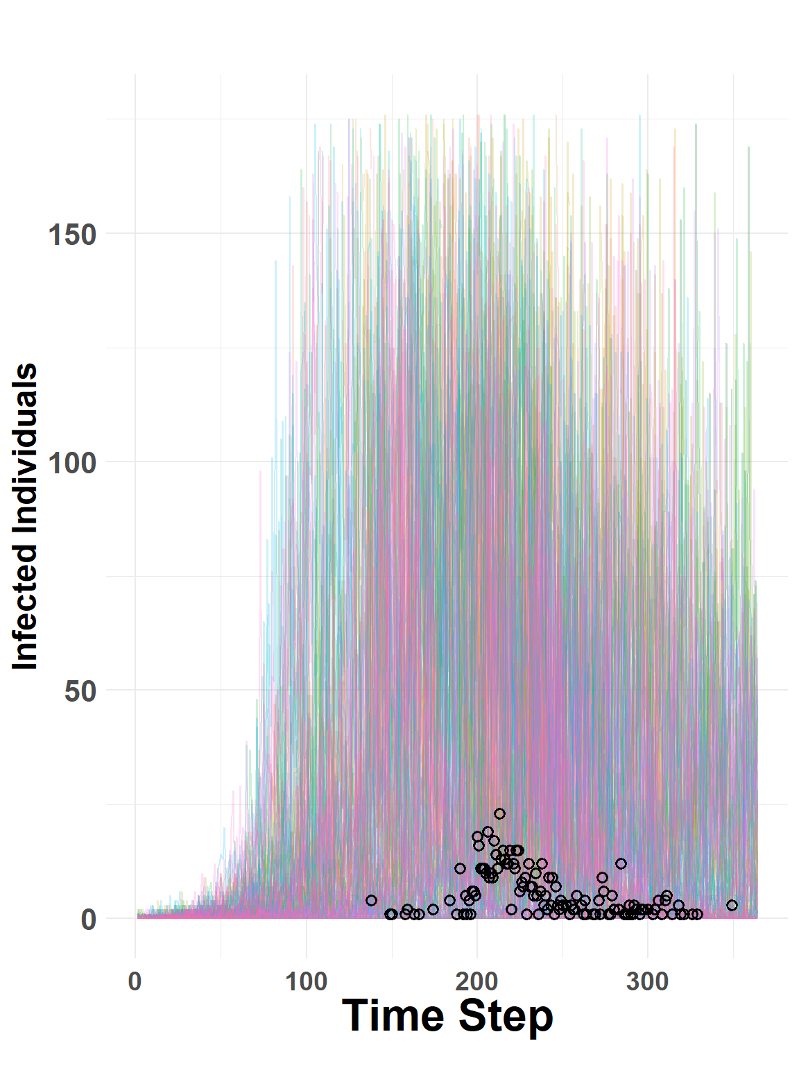
Prior Predictive Distributions The prior model does not have information (data) about the number of observed number of VS cases, therefore predictions here (Figure 5) are based only on incidence as estimated from the SEIR-SEI ODE system and the prior distributions intended to capture mechanistic aspects of VS epidemiology. As a prior predictive check, it’s assumed that predictions will have considerable uncertainty, which is the case in Figure 5, however it is also case that the median counts across the random draws are near the truth.

Hide code

plot_sample_trajectories(prior_model, truth_df=truth_df, n_draws = 100)

Figure 5: Random draws from predictive distribution. Colored lines show sampled trajectories. Height of black points indicate observed daily incidence.

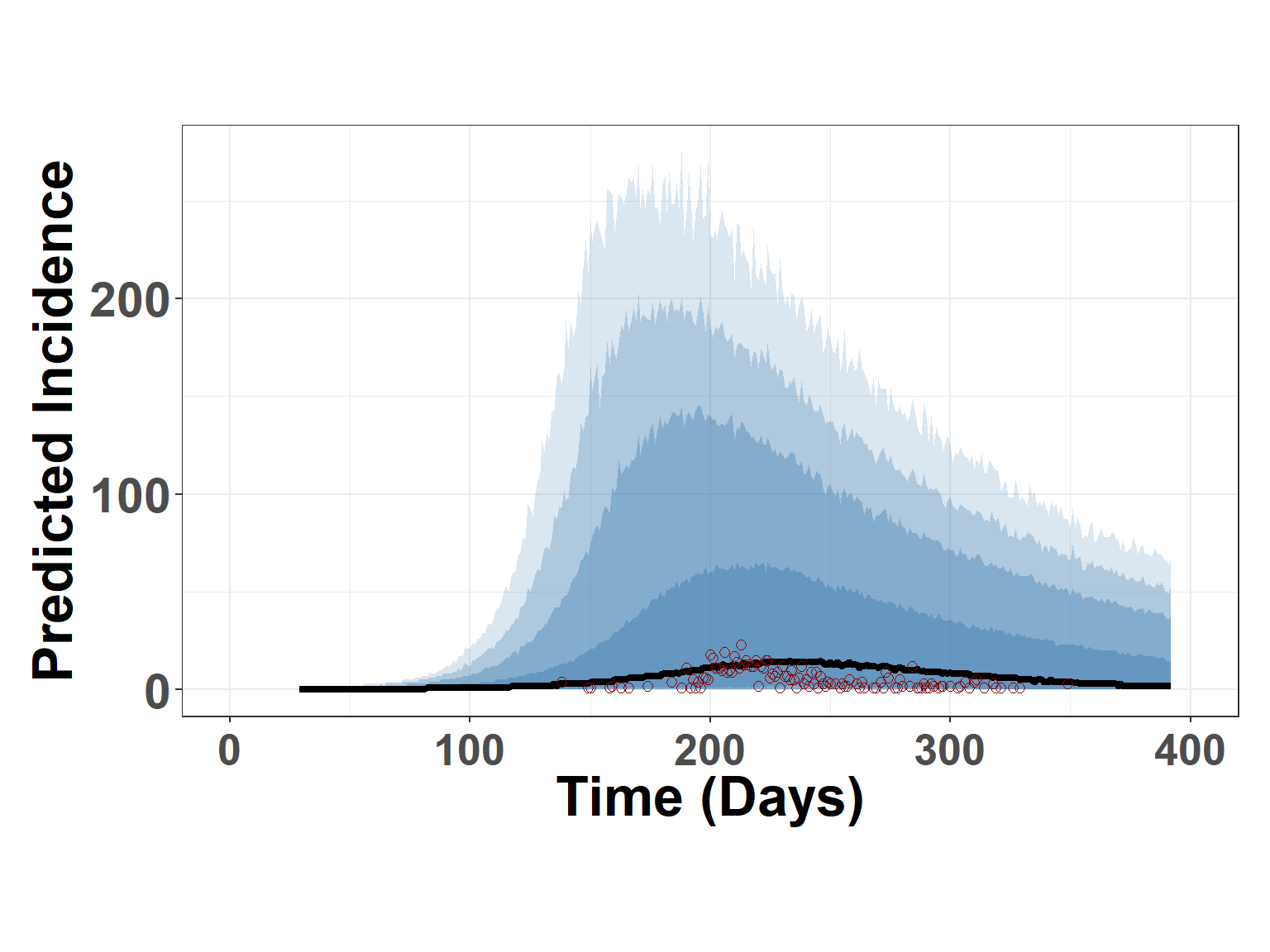
To visualize the prior predictions differently, credible intervals can plotted along with the estimated median prediction (Figure 6).

Hide code

plot_pred_incidence(prior_model, my_truth = truth_df)  

Warning: Using `size` aesthetic for lines was deprecated in ggplot2 3.4.0.
ℹ Please use `linewidth` instead.

Figure 6: Figure displays summary credible intervals (blue shading) and median prediction from the prior predictive model. Height of red points indicate observed daily incidence.

Full Bayesian Model

Although parameter values from the prior model are reasonable based on current understanding of VS epidmiology, draws from the prior predictions show far too much uncertainty to have confidence in the model.

To improve the model, the Stan code is updated to include the following elements:

Observed Incidence
The data block shown in the code is modfied to take observed incidence as an input. The observed incidence is referred to as cases in the code.

data {
...
int cases[n_days];
}

The model block is revised to include the observed cases when sampling from the NegBinomial.

model {
...
cases[1:(n_days-1)] ~ neg_binomial_2(incidence, phi);
}

Observation Bias
In addition to incorporting observed incidence, the model a new model parameter is added to account for underreporting and other possible errors in the observations. The bias parameter is designated as \kappa and used to reduce incidence as estimated by the SEIR-SEI system.

The new \kappa parameter in the transformed parameters block,

transformed parameters{
...
for (i in 1:n_days-1){
    incidence[i] = -(y[i+1, 2] - y[i, 2] + y[i+1, 1] - y[i, 1])*kappa;
  }

}

and the \kappa prior specification is added to the model block.

model {
  ...
  kappa ~ beta(15, 100);
}

With the addition of \kappa, the previously described sampling distribution (Equation 2) becomes, \begin{align} \nonumber \text{Y}_{t}|\theta &\sim \text{NegBinomial}(\text{Y}|\Delta\text{I}_{t}\bold{\kappa}, \phi) \\ \nonumber \end{align}

Pointwise Log-Likelihood
Lastly, code is added to the generated quantities block to facilitate some checks after the model is run.

generated quantities{
...
real log_lik[n_days-1];
  
  for (i in 1:(n_days - 1)) {
    log_lik[i] = neg_binomial_2_lpmf(cases[i] | incidence[i], phi);
  }
}

The Stan code for the full Bayesian model, with the revisions decribed above can be viewed here: Full SEIR-SEI Model

Full Bayesian model results

Download the executed model object for 2014 VS Outbreaks

Hide code

fit_2014 <- get_data_osf("fit_2014")

File downloaded successfully and saved as fit_2014.rds 

Figure 7 provides posterior predictive checks for the full model for comparison to the prior model Figure 5.

Hide code

plot_sample_trajectories(fit_2014, truth_df=truth_df, n_draws = 100, ymax_prob = 1)

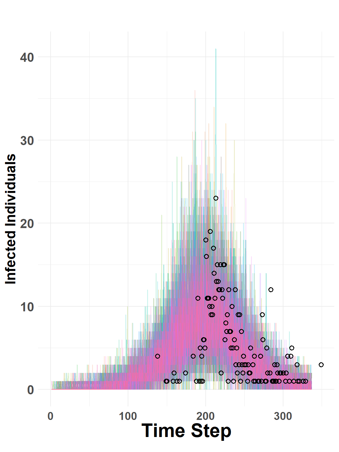
Figure 7: Random draws from posterior predictive distribution. Colored lines show sampled trajectories. Height of red circles indicate observed daily incidence.

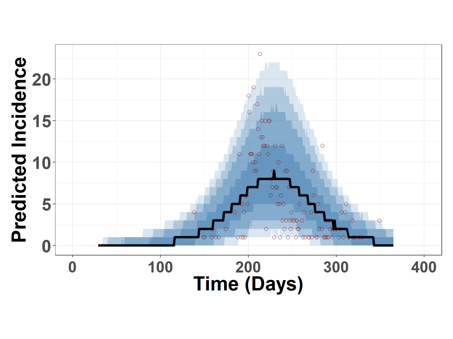
To visualize the prior predictions differently, (Figure 8) displays credible intervals with the estimated median as shown for the prior model (Figure 6).

Hide code

plot_pred_incidence(fit_2014, my_truth = truth_df)  

Figure 8: Figure displays summary credible intervals (blue shading) and median prediction from the prior predictive model. Height of red points indicate observed daily incidence.

Diagnostics

Please see the Diagnostics tab on this website for additional model checks.