Diagnostics

Synopsis

This page demonstrates several diagnostic checks of the models presented in the paper. Please see the Overview tab on this website to view a brief model tutorial.

Load Full Models

Executed model objects are approximately 200mb in size and are archived at the project’s Open Science Framework site HERE.

Hide code

fit_2014 <- get_data_osf("fit_2014")

File downloaded successfully and saved as fit_2014.rds

Hide code

fit_2015 <- get_data_osf("fit_2015")

File downloaded successfully and saved as fit_2015.rds

Check Divergences and Acceptance Rates

No issues or concerns here. Acceptance rate is a little high (above 0.8), but tree depth is good (well below 10), and there are no model divergences.

Hide code

# extract sampler metrics
sampler_merics_2014 <- get_sampler_params(fit_2014, inc_warmup = FALSE)
sampler_merics_2015 <- get_sampler_params(fit_2015, inc_warmup = FALSE)

# 2014 divergences, treedepth, and acceptance rate by chain
sapply(sampler_merics_2014, function(x) mean(x[, "divergent__"]))

[1] 0 0 0 0

Hide code

sapply(sampler_merics_2014, function(x) mean(x[, "treedepth__"]))

[1] 5.9965 6.0390 6.2970 6.1960

Hide code

sapply(sampler_merics_2014, function(x) mean(x[, "accept_stat__"]))

[1] 0.9206312 0.9301491 0.9519151 0.9410590

Hide code

# 2015 divergences, treedepth, and acceptance rate by chain
sapply(sampler_merics_2015, function(x) mean(x[, "divergent__"]))

[1] 0 0 0 0

Hide code

sapply(sampler_merics_2015, function(x) mean(x[, "treedepth__"]))

[1] 5.9885 5.9225 5.9695 5.9155

Hide code

sapply(sampler_merics_2015, function(x) mean(x[, "accept_stat__"]))

[1] 0.9609815 0.9337307 0.9504317 0.9404932

\hat{R} Statistic

All \hat{R} values are approximately 1.0. One approach to checking if a chain has converged to the equilibrium distribution is by comparing its behavior with other chains that were initialized randomly. The (\hat{R}) statistic calculates the ratio of the average variance of samples within each chain to the variance of pooled samples across all chains. At equilibrium, these variances should be equal, making \hat{R} equal to one. If the chains have not yet converged to a common distribution, \hat{R} will be greater than one.

Hide code

rhats14 <- rhat(fit_2014)
mcmc_rhat(rhats14) + 
  ggtitle("Rhats for fit_2014")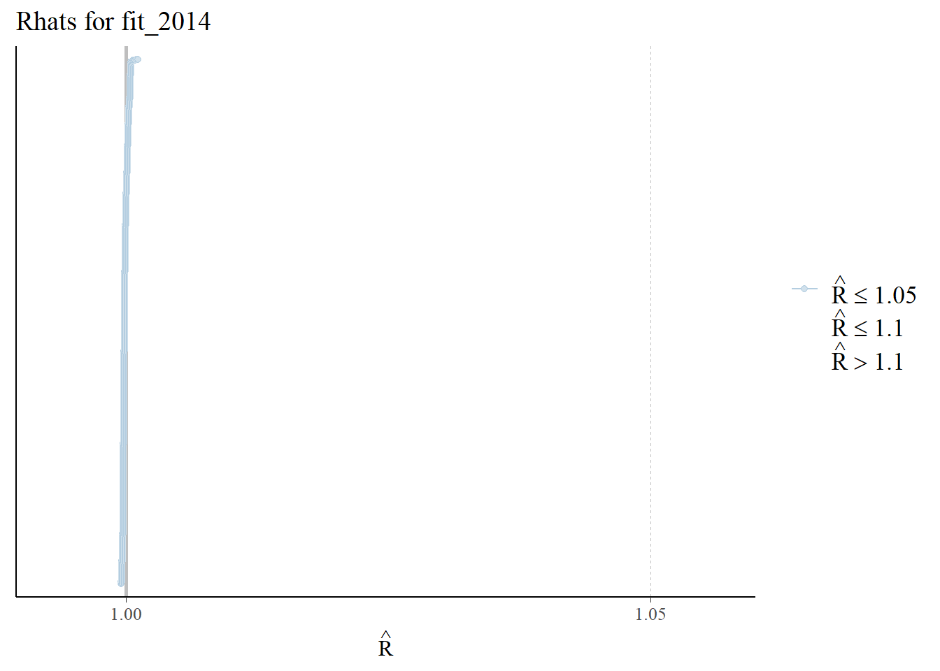

Hide code

rhats15 <- rhat(fit_2015)
mcmc_rhat(rhats15) + 
  ggtitle("Rhats for fit_2015")

Effective Sample Size

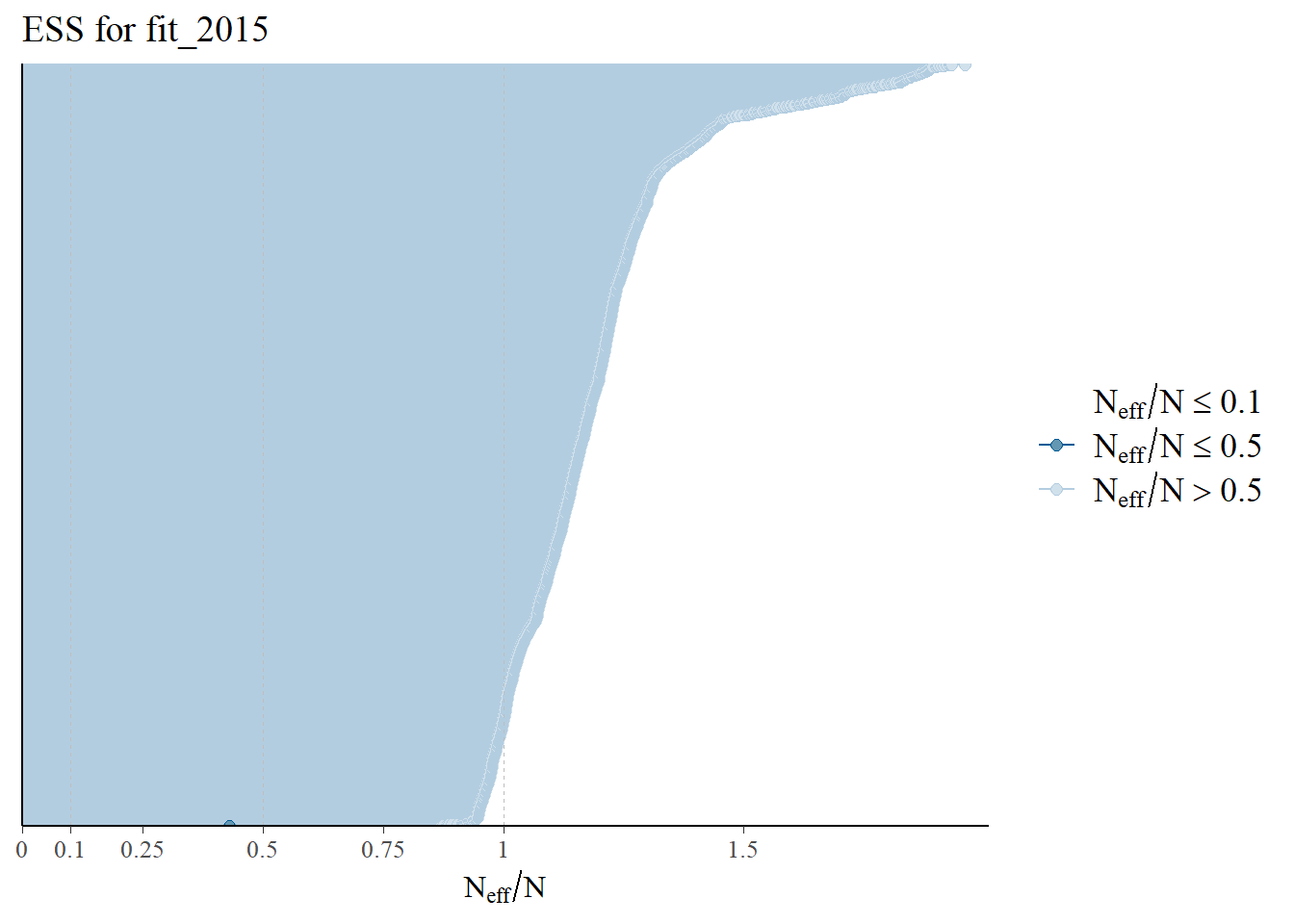
All ESS values are over 0.5. The effective sample size (ESS) estimates the number of independent samples from the posterior distribution. In Stan, the ESS reflects how well the samples can estimate the true mean of a parameter. Due to autocorrelation in a Markov chain, the ESS is usually smaller than the total number of samples (N). If the ESS were less than 0.1, there mighthbe an issue.

Hide code

ratios_cp_14 <- neff_ratio(fit_2014)
mcmc_neff(ratios_cp_14, size = 2) + 
  ggtitle("ESS for fit_2014")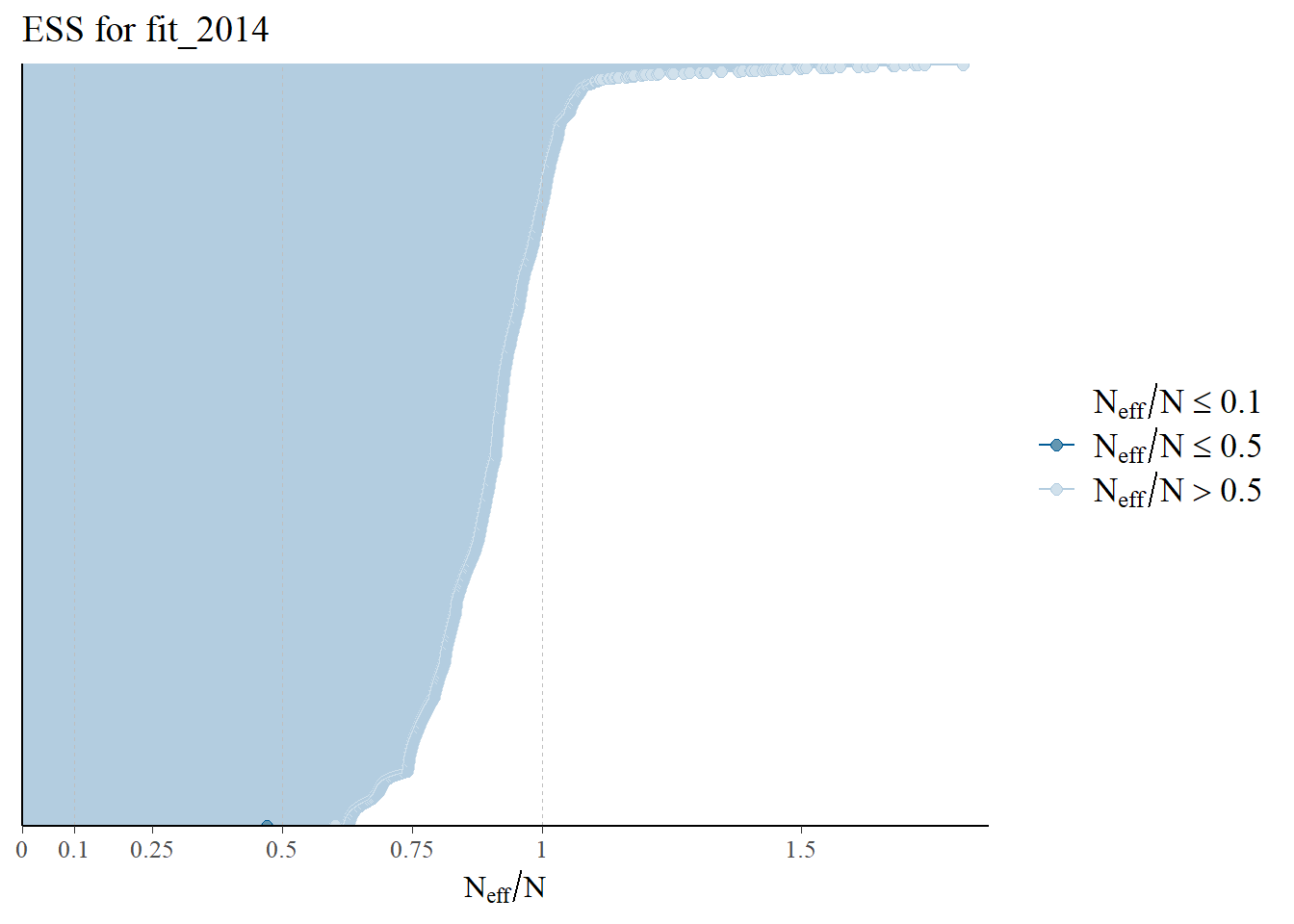

Hide code

ratios_cp_15 <- neff_ratio(fit_2015)
mcmc_neff(ratios_cp_15, size = 2) + 
  ggtitle("ESS for fit_2015")

Model Overview

Please see the Overview tab to view a model construction tutorial.