Identify and Trace Plume Emission Source

HPAI

Spatiotemporal

Published

April 27, 2025

1 Overview

This script provides a conceptual workflow that back traces or verifies the source farm that instigated secondary outbreaks at other farms through atmospheric dispersion of virus. That is, the script looks at data from a secondary outbreak and attempts to determine what source farm emitted the virus that seeded virus introduction. This script moves backward in time to identify the source of a pathogenic plume.

The companion and preceding script for this analysis is available here, Simulated Outbreak. That analysis moves forward in time to model what farms could have been subject to pathogen invasion after plume emission from a source farm. This preliminary script provides a more intuitive overview than the current one which requires a hindsight perspective.

2 Preliminary Setup

Libraries

This workflow uses the renv package for package version and environmental management. The renv.lock file is included to facilitate package installation. See, renv::restore().

Core Functions

Custom functions

Hide code

source(here("R/utilities.R"))
source_dir(here("R"))

Authentication

User credentials to access data repository and API resources.

Hide code

authentications <- yaml::read_yaml(here("local", "secrets.yaml"))

API Registration

Stadia maps are used for backgrounds.

Hide code

register_stadiamaps(key = authentications$stadi_api)

OSF Link

Models and data generated from this script are stored at the Open Science Framework (OSF) for remote access. See, this OSF Project:

Hide code

osf_auth(authentications$osf_token) # for write/admin privileges

Registered PAT from the provided token

Hide code

osf_project_demo <- osf_retrieve_node("https://osf.io/su4yz/")

osf_project_demo$name # scratch directory on OSF EpiPlume project

[1] "Demonstration Data"

3 Read Configuration Parameters

Parameters for epidemiological and spatial analyses are recorded in configuration files. Loading the demonstration config file, which can be viewed here: Demo Configuration Parameters.

Hide code

cfg <- yaml::read_yaml(here("config", "demo_2025-04-21.yaml"))

4 Simulated Outbreak

Downloading and reading the data frame resulting from forward simulation in the Simulated Outbreak script. This file has the coordinates and outbreak detection date for the secondarily infected farms (only one in this demo run) and source farm.

Hide code

osf_id <- osf_project_demo %>%
  osf_ls_files() %>%
  filter(name == "demo_outbreak_sim_2025-04-28.csv")

osf_download(osf_id,
             path = here("local/temp"),
             conflicts = "overwrite")

name	id	local_path	meta
demo_outbreak_sim_2025-04-28.csv	680faa9b91b1af0e5e7c5bb0	local/temp/demo_outbreak_sim_2025-04-28.csv	demo_outbreak_sim_2025-04-28.csv , file , /680faa9b91b1af0e5e7c5bb0 , 1414 , osfstorage , /demo_outbreak_sim_2025-04-28.csv , 1745857179 , 1745857179 , 13361dc0fd02ffb1c1b27224e97d7469 , 1201290c6e31d84d575f9ad16d5c62ce9de5b16256a4d125933476e7bd3a7833 , 0 , TRUE , 1 , FALSE , https://api.osf.io/v2/files/680faa9b91b1af0e5e7c5bb0/ , https://files.osf.io/v1/resources/su4yz/providers/osfstorage/680faa9b91b1af0e5e7c5bb0 , https://files.osf.io/v1/resources/su4yz/providers/osfstorage/680faa9b91b1af0e5e7c5bb0 , https://files.osf.io/v1/resources/su4yz/providers/osfstorage/680faa9b91b1af0e5e7c5bb0 , https://osf.io/download/680faa9b91b1af0e5e7c5bb0/ , https://mfr.osf.io/render?url=https%3A%2F%2Fosf.io%2Fdownload%2F680faa9b91b1af0e5e7c5bb0%2F%3Fdirect%26mode%3Drender, https://osf.io/su4yz/files/osfstorage/680faa9b91b1af0e5e7c5bb0 , https://api.osf.io/v2/files/680faa9b91b1af0e5e7c5bb0/ , https://api.osf.io/v2/files/680c0182fd8f8cdc22d2b775/ , 680c0182fd8f8cdc22d2b775 , files , https://api.osf.io/v2/files/680faa9b91b1af0e5e7c5bb0/versions/ , https://api.osf.io/v2/nodes/su4yz/ , su4yz , nodes , https://api.osf.io/v2/nodes/su4yz/ , nodes , nodes , su4yz , https://api.osf.io/v2/files/680faa9b91b1af0e5e7c5bb0/cedar_metadata_records/

Hide code

simulated_outbreaks <- read.csv(here("local/temp/demo_outbreak_sim_2025-04-28.csv")) %>%
  filter(!is.na(outbreak)) # keeping only farms that experienced outbreak

Convert to Points

Data frame to spatial points

Hide code

# Long/Lat
farm_points_wgs84 <- vect(simulated_outbreaks,
                          geom = c("x", "y"),
                          crs = "EPSG:4326")

Get metadata for simulated farms

Hide code

outbreak_farm_meta <- as.data.frame(farm_points_wgs84, geom="xy") %>%
  filter(name != "source_farm") %>%
  select(-X) # row names

orig_source_meta <- as.data.frame(farm_points_wgs84, geom="xy") %>%
  filter(name == "source_farm") %>%
  select(-X)

5 Create Study Area

Defining a study area extent (raster grid) with the secondary outbreak farm at center. The original source farm is also depicted as reference. The define_study_domain() identifies the appropriate UTM and returns projected objects.

Hide code

study_area_args <- c(
  list(
    source_origin = c(outbreak_farm_meta$x, outbreak_farm_meta$y),
    extent_km = cfg$domain$extent_km,
    res_m = cfg$domain$res_m  
  )
)

study_area <- exec(define_study_domain, !!!study_area_args)

# projected UTM
farm_points <- project(farm_points_wgs84, crs(study_area$projection))

Plot study area

The circle at center is the secondarily infected farm; the goal is to look backward in time to demonstrate that the source farm (triangle, lower right) emitted the plume that gave rise to the outbreak at the center.

Hide code

map_grid(study_area$grid, source_loc = farm_points)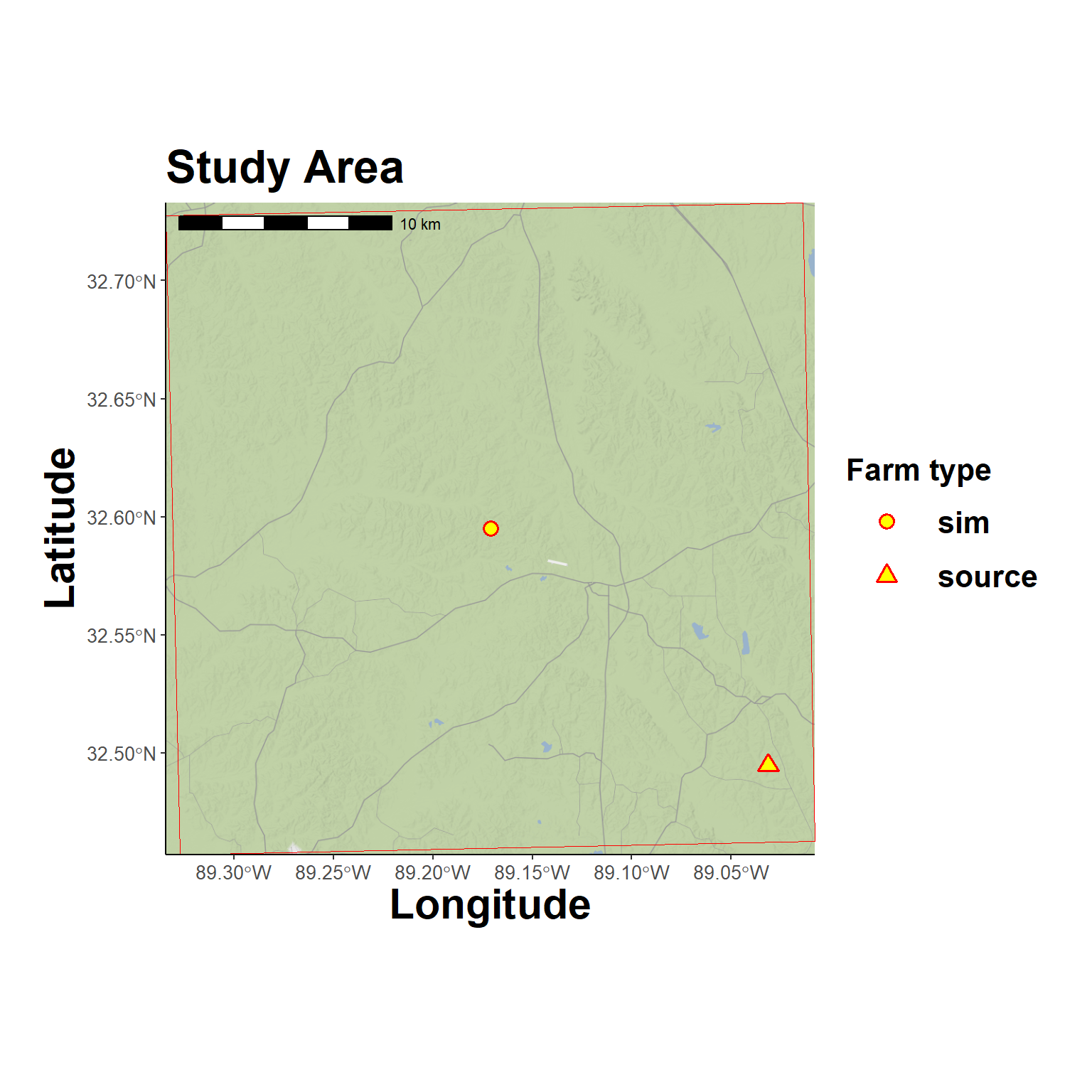

6 Trajectory Models

A HYSPLIT model is constructed assuming the secondary outbreak location was a receptor of the plume from an unknown source. The splitR package is used to call a HYSPLIT executable from R.

Time limit to download meteorological data.

Hide code

getOption("timeout")

[1] 60

Hide code

options(timeout=10000)

Date Determination

Determine dates and times to evaluate. Although it is known when the outbreak was detected at the secondary farm, it is not known when the virus was introduced nor when initial infection occurred. In practice, poultry workers would likely only detect an outbreak once the rate of daily chicken mortality sufficiently and consistently (multiple days) exceeded that typical background rate. In this example, it’s assumed that latent periods and initial spread from a single chicken took at least 3 days (earliest possible detection), but may have taken 20 days to detect. Therefore, this demo analyses more than two weeks in the past.

Hide code

model_name <- gsub("_", "", outbreak_farm_meta$name) # 6 characters max
model_name

[1] "farm18"

Hide code

earliest_date <- as_date(outbreak_farm_meta$outbreak) - days(20) # assuming slow to detect
latest_date <- as_date(outbreak_farm_meta$outbreak) - days(3) # allowing for at least 2 day latent period and 1 day infectious

dates_to_check <- seq(earliest_date, latest_date, by = 1)
length(dates_to_check) # total days to model

[1] 18

Run Trajectory Model

The wrap_trajectory_model() saves locally, but a copy is also saved to OSF for others to use. There are a ton of parameter assumptions here to discuss. Brief explanations are provided with the config file (linked here), but its too much for this draft workflow.

This model estimates four trajectories per day (every 6 hours) for each of the 18 days, for a a total of 72 trajectories.

Hide code

traj_model <- wrap_trajectory_model(cfg, # configuration file
                                    traj_name = model_name,
                                    lon = outbreak_farm_meta$x, # simulated outbreak farm
                                    lat = outbreak_farm_meta$y, # simulated outbreak farm
                                    height = cfg$trajectory$traj_height,
                                    duration = cfg$trajectory$traj_duration,
                                    days = dates_to_check, # days to assess based on simulated outbreak timeline
                                    daily_hours = cfg$trajectory$daily_hours,
                                    model_height = cfg$trajectory$model_height, 
                                    direction = cfg$trajectory$traj_direction,
                                    extended_met = cfg$trajectory$extended_met,
                                    vert_motion = cfg$trajectory$vert_motion,
                                    met_type = cfg$trajectory$traj_met_type,
                                    met_dir = here(cfg$trajectory$traj_climate),
                                    exec_dir = here(cfg$trajectory$traj_outputs),
                                    clean_up = cfg$trajectory$traj_clean_up
                                )

# save copy to OSF
osf_upload(osf_project_demo, path = here("local/demo_run/traj/farm18_model.rds"))

Download trajectory model from OSF (if not run locally)

Hide code

osf_id <- osf_project_demo %>%
  osf_ls_files() %>%
  filter(name == "farm18_model.rds")

osf_download(osf_id,
             path = here("local/temp"),
             conflicts = "overwrite")

Read the pre-run trajectory model

Hide code

traj_model <- readRDS(here("local/temp/farm18_model.rds"))

Plot hindcast trajectories

Each line is a trajectory extending from the secondarily infected farm (center) that follows atmospheric characteristics for the hind cast date and time. This plot shows the complete trajectory.

Hide code

map_grid2(study_area$grid, traj_model$traj_df, group_col = "run", vector_type = "line", grid_cut = FALSE)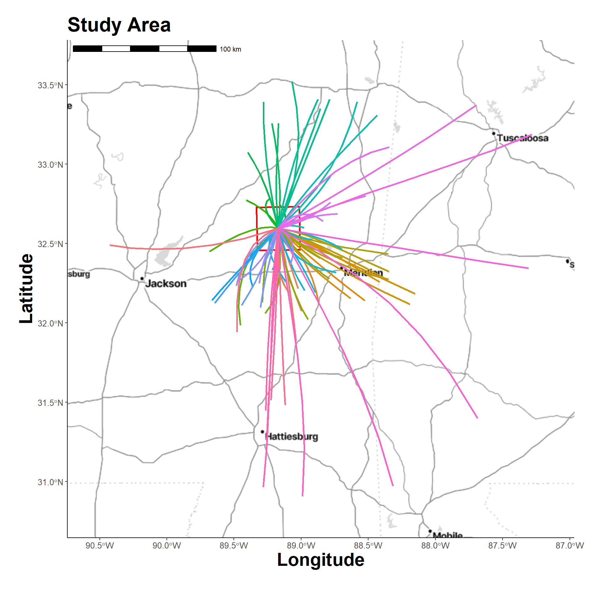

The trajectories in this plot are cropped to the extent of study area with option grid_cut to better see individual paths.

Question: Do any of these trajectories help identify and confirm the source farm?

Hide code

map_grid3(study_area$grid, traj_model$traj_df, group_col = "run", vector_type = "line", source_loc = farm_points_wgs84, grid_cut = TRUE)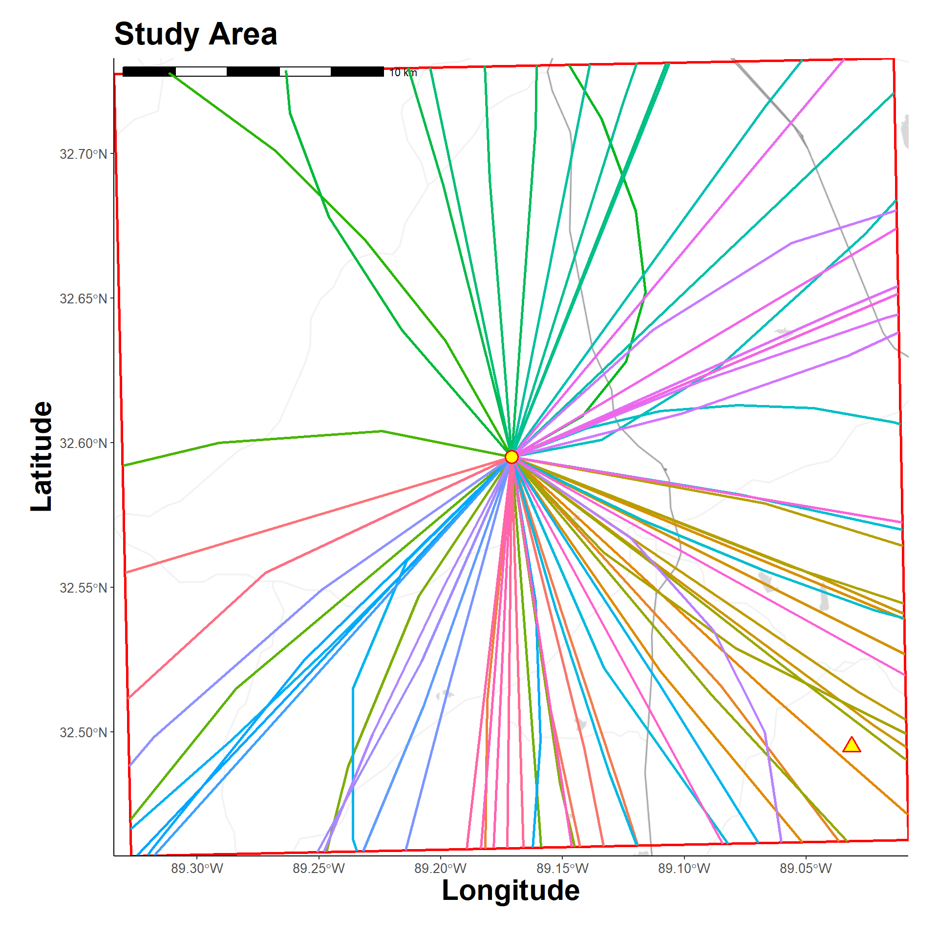

7 Spatial Analysis

A couple basic steps to compare distances between the source farm and possible trajectories from the secondary outbreak farm.

Measure distances

The measure_proximity() function measures distances for both the trajectory lines and point outputs.

Hide code

traj_dists <- measure_proximty(
  target_location = c(orig_source_meta$x, orig_source_meta$y), # suspected source farm
  traj_model = traj_model,
  projection = study_area$projection
  )

Inverse Distance Decay

Apply an inverse distance decay function assuming that trajectory probability decreases the further from the source farm it is:

w(d) = \exp(-\lambda \times d)
where:
- w(d) is the weight (between 0 and 1),
- d is the distance in meters between the source and the trajectory,
- \lambda is a decay rate parameter, how quickly the weight decreases with distance.

Hide code

distance_threshold <- 10000 # meters, 10k, decreasing probability of trajectory after this distance

lambda_value <- calibrate_lambda(distance_threshold, weight_target = 0.5) # find the best lambda with 10k as the median probability

Show the relationship (green is the lambda_value).

Hide code

plot_distance_decay(
    lambda_target = lambda_value,
    weight_target = 0.5 # median probability
)

Warning: Using `size` aesthetic for lines was deprecated in ggplot2 3.4.0.
ℹ Please use `linewidth` instead.

Warning in geom_hline(yintercept = weight_target, linetype = "dashed", color =
"black", : Ignoring unknown parameters: `linewdith`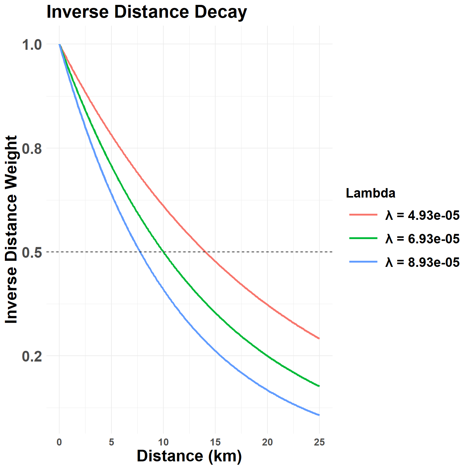

Score and Subset

Calculate the probability for each modeled trajectory

Hide code

traj_dists$traj_lines$score <- calculate_inverse_distance_weight(traj_dists$traj_lines$distance_m, 
                                                                 lambda = lambda_value) # score distances

Select trajectories with at least a 90% probability.

Hide code

closest_traj_line <- as.data.frame(traj_dists$traj_lines) %>%
  filter(score >= 0.9) %>%
  arrange(desc(score)) %>%
  select(run, distance_m, score)

Filter trajectory data to possible distances.

Hide code

runs_50 <- unique(closest_traj_line$run)

possible_dates <- vect(traj_dists$traj_point)
possible_dates <- project(possible_dates, "EPSG:4326" )
possible_dates <- as.data.frame(possible_dates,
                                geom="xy") %>%
  mutate(lon = x, lat = y) %>%
  filter(run %in% runs_50)

The above reduced 72 possible trajectories to 1970-01-07, 1970-01-11, 1970-01-16, 1970-01-17 probable ones. Show here:

Hide code

map_grid3(study_area$grid, possible_dates, group_col = "run", vector_type = "line", source_loc = farm_points_wgs84, grid_cut = TRUE)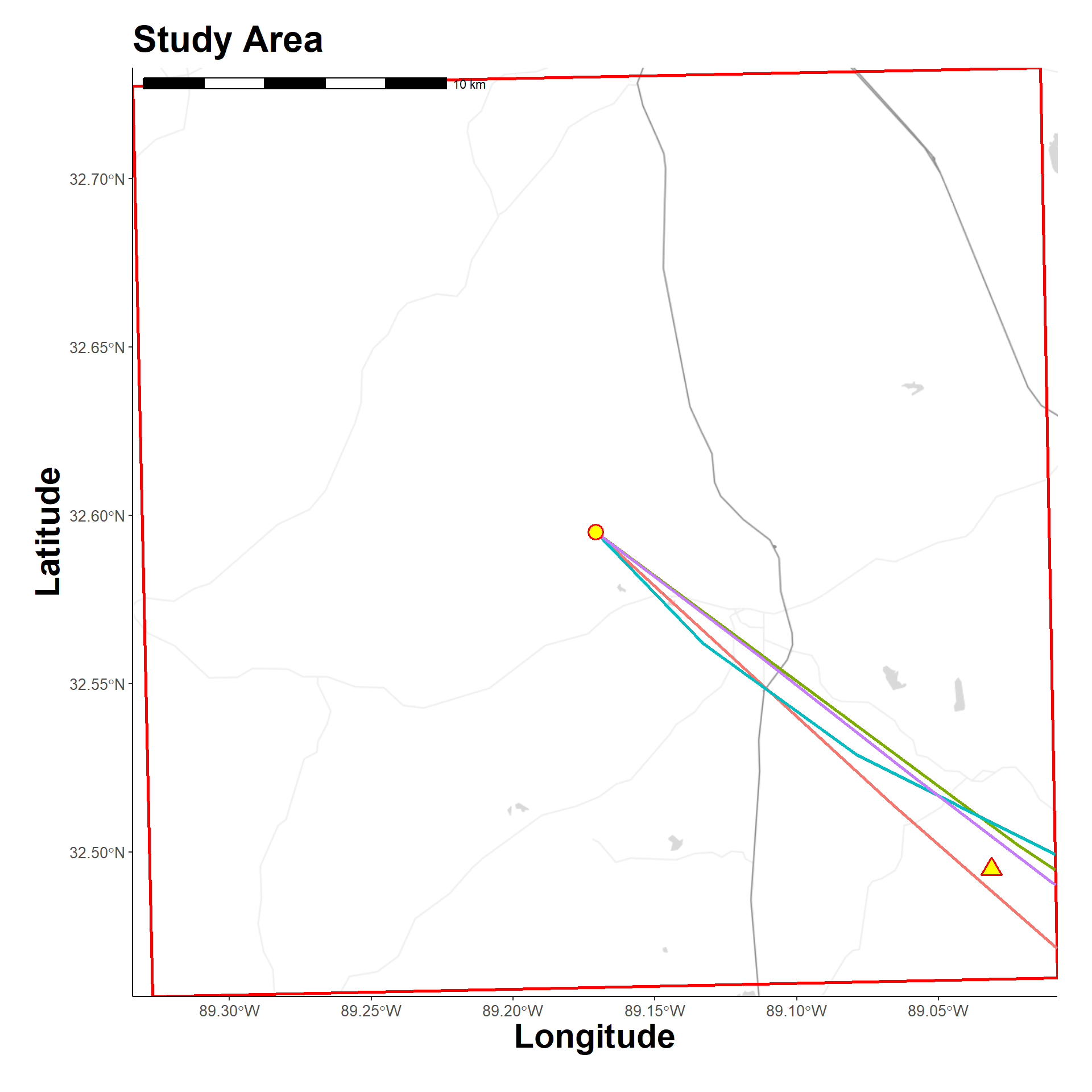

8 Receptor Return

Having narrowed possible trajectory dates and times that could have produced the infecting plume, reverse plumes are simulated from the secondary outbreak farm (receptor) to the original source (backwards in time).

Execute plume model runs in a loop.

Hide code

possible_datetimes <- possible_dates %>%
  mutate(date = as.Date(traj_dt)) %>%
  group_by(date) %>%
  summarise(start = min(traj_dt)) %>%
  as.data.frame()

for(i in 1:unique(possible_datetimes$start)){
  
  plume_name <- paste0("plume_", i)
  
  plume_model <- wrap_plume_model(cfg, # configuration file
                                plume_name = plume_name, # name/label
                                lon = outbreak_farm_meta$x, # secondary outbreak farm
                                lat = outbreak_farm_meta$y, # secondary outbreak farm
                                direction = "backward", # from receptor back in time
                                release_start = possible_datetimes$start[i], # release from source farm
                                release_end = possible_datetimes$start[i] - hours(1), # reverse time
                                start_time = possible_datetimes$start[i], # dispersion time same as emission
                                end_time = possible_datetimes$start[i] - hours(24) # dispersion end
                                )
  
  
  
}

# copy to OSF
osf_upload(osf_project_demo, path = here("local/demo_run/plume/plume_1_model.rds"))
osf_upload(osf_project_demo, path = here("local/demo_run/plume/plume_2_model.rds"))
osf_upload(osf_project_demo, path = here("local/demo_run/plume/plume_3_model.rds"))

Download from OSF

Hide code

osf_id <- osf_project_demo %>%
  osf_ls_files() %>%
  filter(name == "plume_1_model.rds" | 
         name == "plume_2_model.rds" |
         name == "plume_3_model.rds")

osf_download(osf_id,
             path = here("local/temp"),
             conflicts = "overwrite")

Read plume models

Hide code

plume_1 <- readRDS(here("local/temp/plume_1_model.rds"))
plume_2 <- readRDS(here("local/temp/plume_2_model.rds"))
plume_3 <- readRDS(here("local/temp/plume_3_model.rds"))

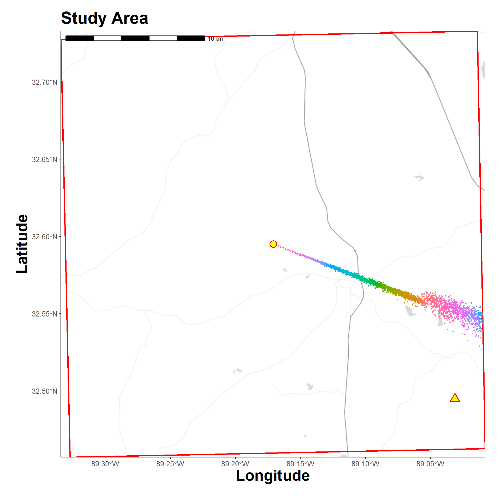
Plume 1 simulated dispersion

Hide code

map_grid3(study_area$grid, plume_1$disp_df, group_col = "particle_i", vector_type = "point", source_loc = farm_points_wgs84, grid_cut = TRUE)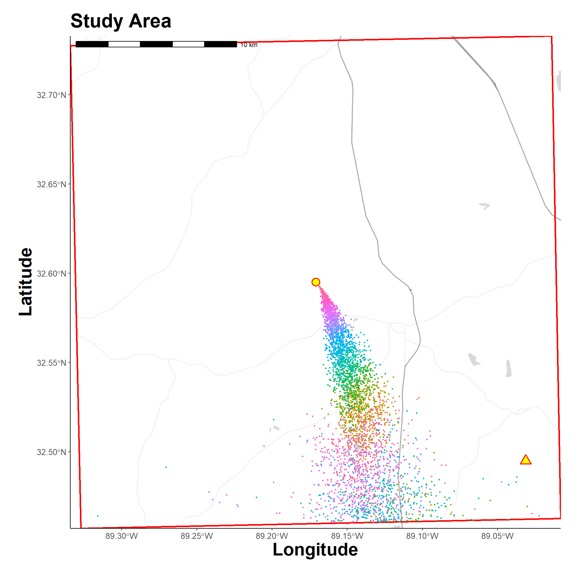

Plume 2 simulated dispersion

Hide code

map_grid3(study_area$grid, plume_2$disp_df, group_col = "particle_i", vector_type = "point", source_loc = farm_points_wgs84, grid_cut = TRUE)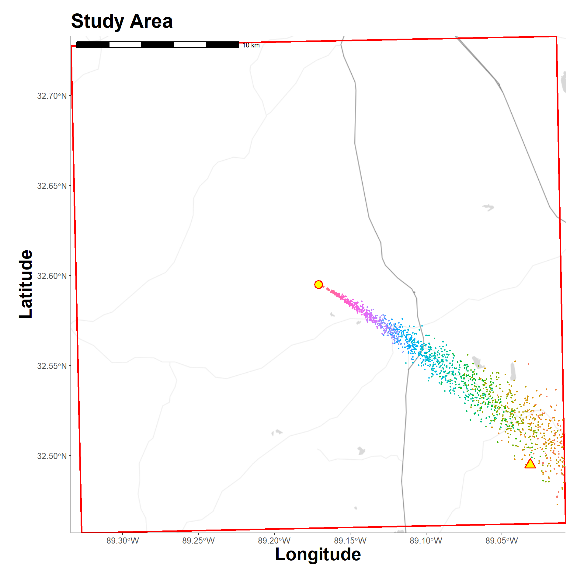

Plume 3 simulated dispersion

Hide code

map_grid3(study_area$grid, plume_3$disp_df, group_col = "particle_i", vector_type = "point", source_loc = farm_points_wgs84, grid_cut = TRUE)