Simulate Airborne Virus Introduction and Outbreak

HPAI

Spatiotemporal

Published

April 27, 2025

1 Overview

This script provides a conceptual workflow that simulates farm locations, performs atmospheric dispersion modeling from a source farm (aka, plume modeling), analyzes the plume results in a spatial temporal model, and then identifies the simulated farms most vulnerable to airborne virus introduction. The results from this forward simulation are analysed in a second script, available here, in an attempt to identify the source farms using only the information from the secondarily infected farms simulated here.

2 Preliminary Setup

Libraries

This workflow uses the renv package for package version and environmental management. The renv.lock file is included to facilitate package installation. See, renv::restore().

Core Functions

Custom functions

Hide code

source(here("R/utilities.R"))
source_dir(here("R"))

Authentication

User credentials to access data repository and API resources.

Hide code

authentications <- yaml::read_yaml(here("local", "secrets.yaml"))

API Registration

Stadia maps are used for backgrounds.

Hide code

register_stadiamaps(key = authentications$stadi_api)

OSF Link

Models and data generated from this script are stored at the Open Science Framework (OSF) for remote access. See, this OSF Project:

Hide code

osf_auth(authentications$osf_token) # for write/admin privileges

Registered PAT from the provided token

Hide code

osf_project_demo <- osf_retrieve_node("https://osf.io/su4yz/")

osf_project_demo$name # scratch directory on OSF EpiPlume project

[1] "Demonstration Data"

3 Read Configuration Parameters

Parameters for epidemiological and spatial analyses are recorded in configuration files. Loading the demonstration config file, which can be viewed here: Demo Configuration Parameters.

Hide code

cfg <- yaml::read_yaml(here("config", "demo_2025-04-21.yaml"))

4 Create Study Area

From a given lat-long, the define_study_domain() function constructs a surrounding square grid at a specified extent and resolution to define a study area. The function optionally generates a specified number of simulated farms. The farms are randomly assigned within the study, based on chicken density estimated in the Gridded Livestock of the World Database (source). The more chickens at a location, the higher the probability that a random farm be placed there. The random farms are assigned a random flock size based on a possible range specified in the config file.

Hide code

study_area_args <- c(
  cfg$domain, # from config
  list(
    seed      = 123,
    min_flock = 15000,
    max_flock = 50000
  )
)

study_area <- exec(define_study_domain, !!!study_area_args)


# attributes
str(study_area)

List of 4
 $ projection  : chr "+proj=utm +zone=16 +north +datum=WGS84 +units=m +no_defs"
 $ grid        :S4 class 'SpatRaster' [package "terra"]
 $ source_point:S4 class 'SpatVector' [package "terra"]
 $ farm_locs   :S4 class 'SpatVector' [package "terra"]

Hide code

# flock sizes
range(study_area$farm_locs$flock)

[1] 15861 49799

flock size at source farm

For the demo, the center most farm used in defining the study area is considered the source of pathogen emission. The flock size is need for that location to estimate emission.

Hide code

source_flock_n <- values(study_area$farm_locs) %>%
  filter(farm == "source") %>%
  select(flock)

source_flock_n

flock
19998

Plot Study Area

The source is the center most triangle, other farms are shown as circles.

Hide code

map_grid(study_area$grid, source_loc = study_area$farm_locs)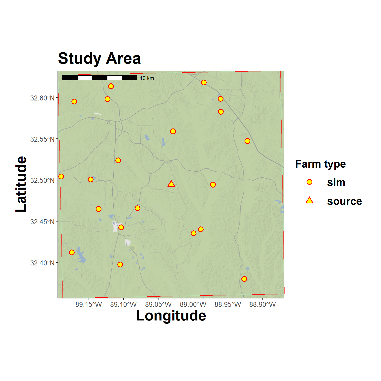

Figure 1: Study area for analysis with simulated farms as indicated in legend.

5 Simulate Outbreak

Dates

Random dates for initial infection and virus emission from the source farm. Assuming detection occurs 5 to 20 days after outbreaks start. That is, when workers notice that chicken death rates are exceeding the normal background rate.

Hide code

sim_dates <- random_infect_dates(year = 2020, month = 5, seed=1976)
sim_dates

$release_date
[1] "2020-05-27"

$infection_date
[1] "2020-05-15"

SEIR and Emission Estimates

Run SEIR model for source farm. There are a ton of parameter assumptions here to discuss. Brief explanations are provided with the config file (linked here), but far too much to include in this draft workflow.

Hide code

# virus decay, rate of decreasing viability
halflife <- calculate_half_life(viability_days = cfg$virus$viability_hours/24, # convert hours to days
                                viability_threshold = cfg$virus$viability_threshold)

args <- list(
  beta       = cfg$seir$beta,
  sigma      = 1 / cfg$seir$sigma, # per/day
  gamma      = 1 / cfg$seir$gamma, # per/day
  qV         = cfg$virus$qV,
  Vh         = cfg$poultry$house_vol,
  Q          = cfg$poultry$Q_m3_h * 24, # to days
  lamd       = log(2) / halflife, # virus decay
  flock_size = source_flock_n$flock, # flock size at source farm
  Ei         = cfg$seir$Ei,
  Ii         = cfg$seir$Ii,
  Ri         = cfg$seir$Ri,
  Vi         = cfg$seir$Vi,
  sim_days   = cfg$seir$sim_days,
  infect_date = sim_dates$infection_date # initial infection
)

seir_out <- do.call(model_seir_shedding, args)

Get rate on day of emission

Hide code

# values for emission day
source_rate <- seir_out %>%
  filter(datetime >= sim_dates$release_date & datetime < (sim_dates$release_date + days(1))) 

# range day of release
range(source_rate$V)

[1] 30.43649 48.47731

View SEIR Dynamics

Top panel is SEIR result, bottom is estimated virus output at the the source farm.

Hide code

plot_ode_shed_dynamics(seir_out, date_axis = TRUE, vline = sim_dates$release_date, vline_text = "Emission")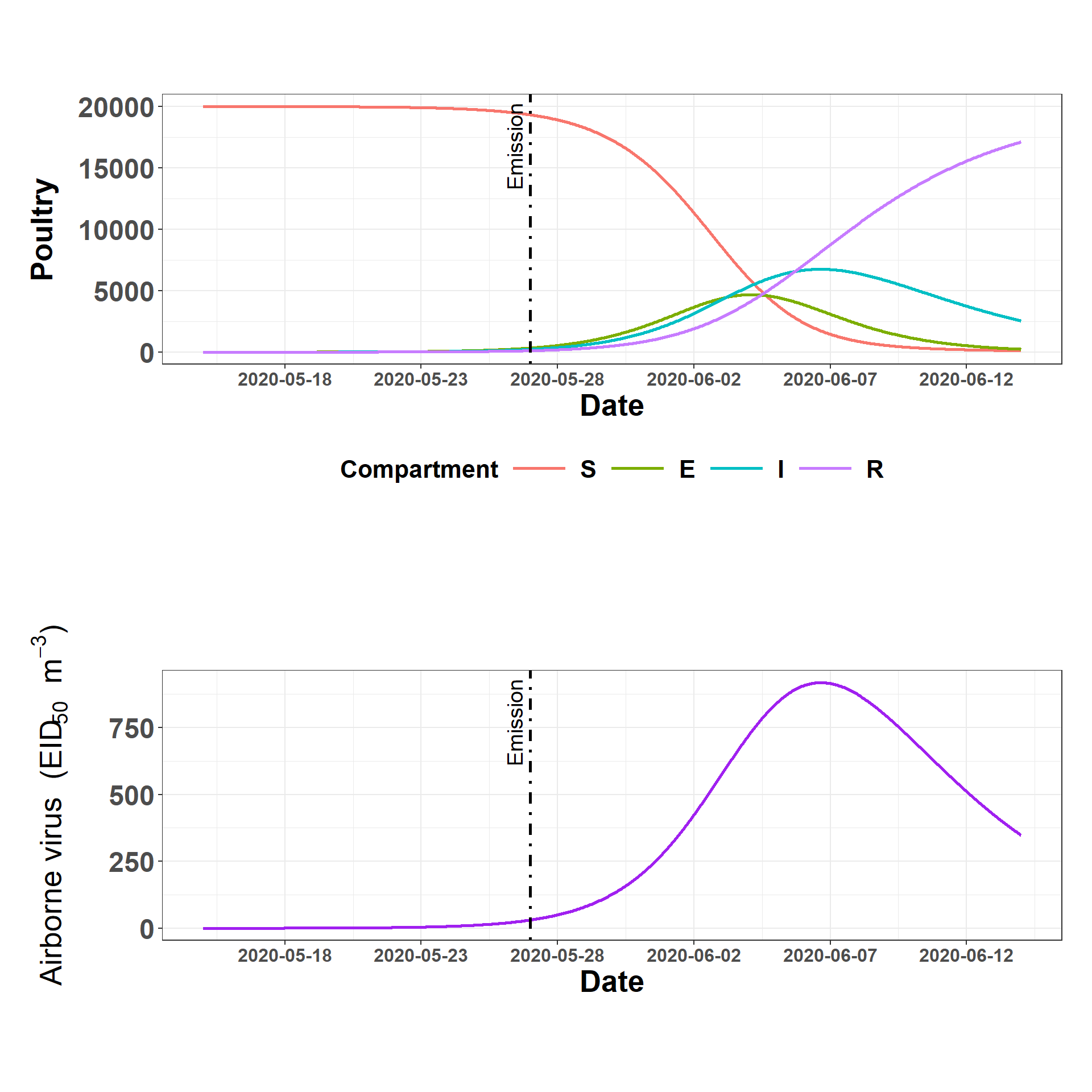

6 Plume Dispersion

A HYSPLIT model is constructed based on the simulated outbreak and source farm emission dynamics. The splitR package is used to call a HYSPLIT executable from R.

Hide code

arbitrary_hour <- 12 # noon
simulated_realease_dt <- ymd_hm(paste0(sim_dates$release_date, " ", sprintf("%02d:00", arbitrary_hour)))

Run plume model

The wrap_plume_model() function saves the plume model locally, however, a copy is also saved to OSF. There are a ton of parameter assumptions here to discuss. Brief explanations are provided with the config file (linked here), but its too much for this draft workflow.

Hide code

plume_model <- wrap_plume_model(cfg, # configuration file
                                plume_name = "sim_demo", # name/label
                                rate = mean(source_rate$V), # rate from simulated outbreak
                                release_start = simulated_realease_dt, # release from source farm
                                release_end = simulated_realease_dt + hours(1), # hour long
                                start_time = simulated_realease_dt, # dispersion time same as emission
                                end_time = simulated_realease_dt + hours(24) # dispersion end
                                )

# copy to OSF for others to access (~500kb)
osf_upload(osf_project_demo, path = here("local/demo_run/plume/sim_demo_model.rds"))

Download plume model from OSF

Hide code

osf_id <- osf_project_demo %>%
  osf_ls_files() %>%
  filter(name == "sim_demo_model.rds")

osf_download(osf_id,
             path = here("local/temp"),
             conflicts = "overwrite")

Read plume model

Hide code

plume_model <- readRDS(here("local/temp/sim_demo_model.rds"))

View complete simulated dispersion

Full extent of plume

Hide code

map_grid2(study_area$grid, plume_model$disp_df, group_col = "particle_i", vector_type = "point", grid_cut=FALSE)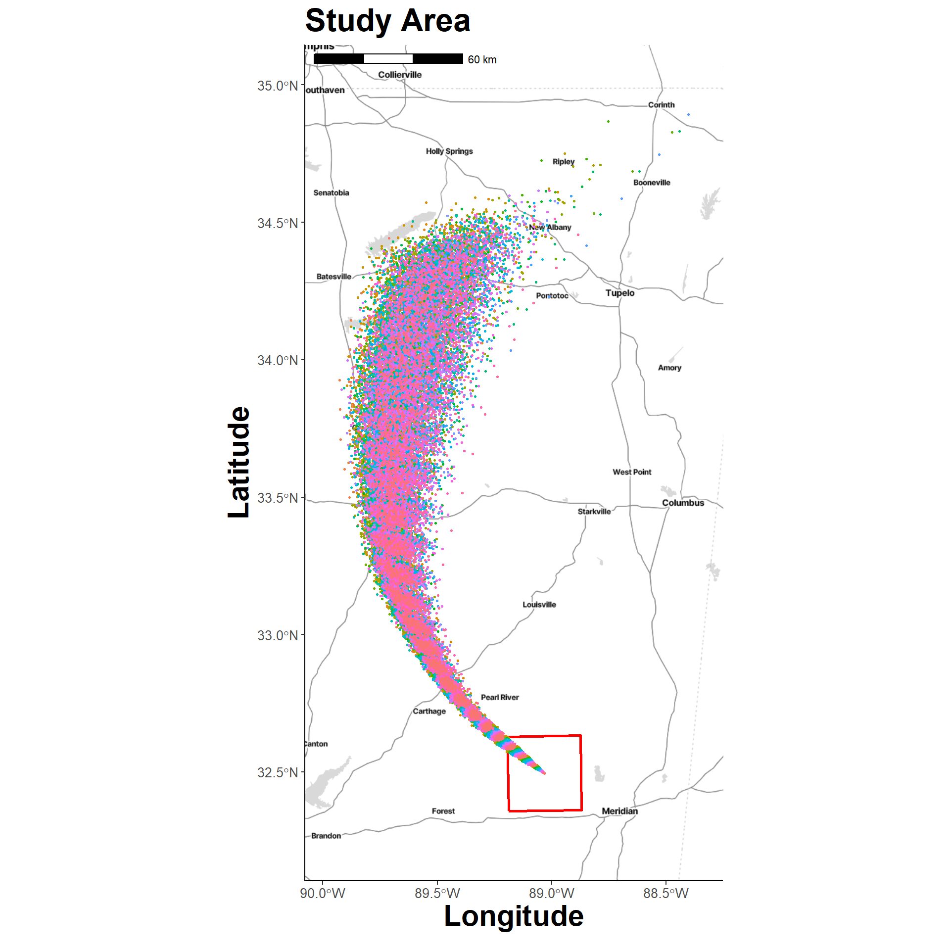

Plume extent within study area

Hide code

map_grid2(study_area$grid, plume_model$disp_df, group_col = "particle_i", vector_type = "point", grid_cut=TRUE)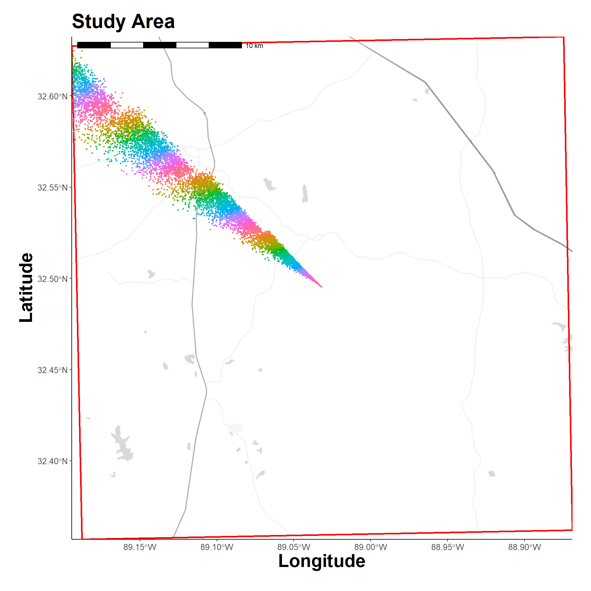

A quick, low-weight animation as a spot check of time.

Hide code

animate_disp <- animate_plume_simple(traj_data = plume_model$disp_df, 
                                     group_col = "particle_i", 
                                     point_size = 0.5, 
                                     source_loc=cfg$domain$source_origin)

Hide code

knitr::include_graphics(here("assets/plume_animation2.gif"))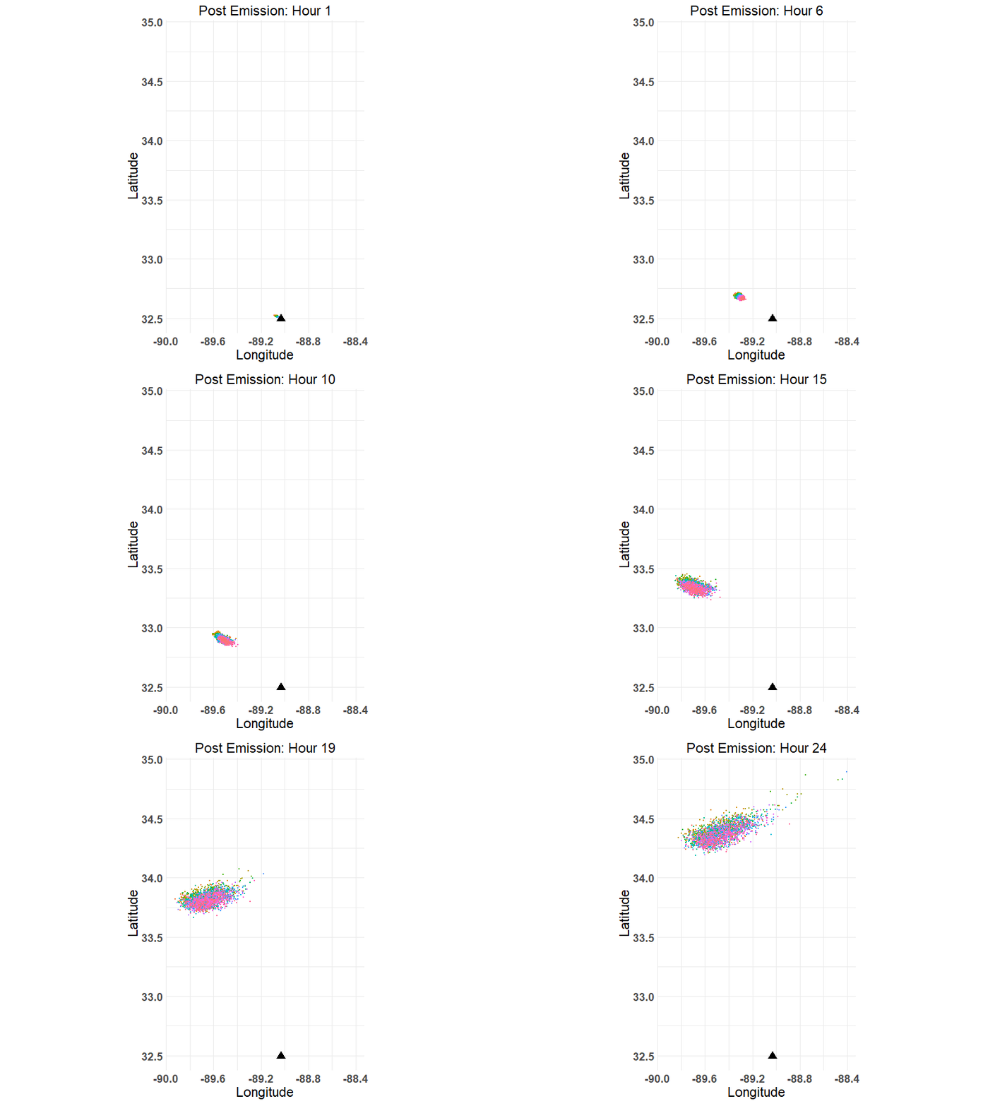

7 Calculate Concentration

The calculate_particle_concentration() utilizes HYSPLIT estimated particles to calculate the particles per m3 hour. Limiting analysis to first 6 hours, beyond that time the plume is outside the study area.

Hide code

concentration_lst <- calculate_particle_concentration(plume_table=plume_model$disp_df, 
                                                      raster_grid = study_area$grid,
                                                      voxel_height = 50, # height (m)
                                                      max_hour = 6) # maximum hour to use

View Concentration

Viewing the first hour only.

Hide code

check_hour <- 1

map_grid(study_area$grid, 
         source_loc = study_area$source_point, 
         concentration_raster = concentration_lst$concentration_stack[[check_hour]],
         map_type = "stamen_toner_lite")

ℹ © Stadia Maps © Stamen Design © OpenMapTiles © OpenStreetMap contributors.

Coordinate system already present. Adding new coordinate system, which will
replace the existing one.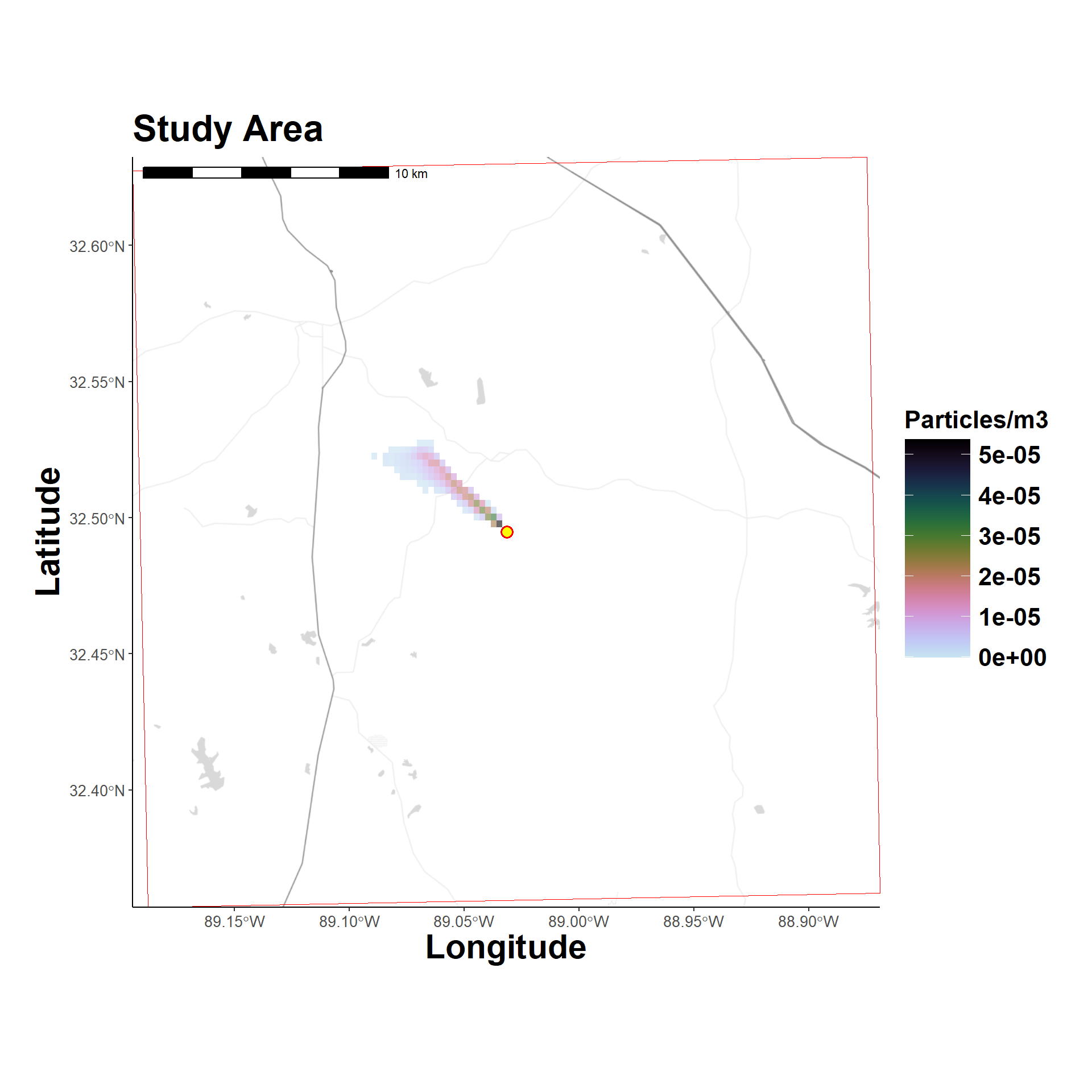

Get concentration estimates for later analysis.

Hide code

concentration_df <- as.data.frame(concentration_lst$concentration_stack, xy = TRUE)

conc_melt <- reshape2::melt(concentration_df, c("x","y"))

conc_melt$hour <- as.integer(sub("^hour_", "", conc_melt$variable))

conc_melt <- conc_melt %>%
  mutate(hour = as.integer(sub("^hour_", "", variable)),
         concen = value) %>%
  select(-c(variable, value))

8 Spatiotemporal Modeling

The primary objective of spatial modeling is to account for spatial (s) and temporal (t) latency (error, variability) and uncertainty in HYSPLIT outputs. This smoothed results and enables uncertainty estimation. Just as importantly, developing the the HYSPLIT outputs to a spatiotemporal model allow for incorporating other variables, to include climate, land cover, farm specific biosecurity factors, and genetic samples to name a few.

The modeling framework here is a two-tiered joint model that concurrently estimates particle counts (tier 1, {y}_{1st}) and mass concentration (tier 2, {y}_{2st}) while accounting for correlated spatial and temporal factors as well as their interaction. These analyses follow a point-process framework, however concentration points in {y}_{2st} actually represent an area (grid cell). To help account for errors created when aggregating particles to grid cells, the random spatial field from the individual particles is shared with tier 2. In essence, individual particles act as a predictor or covariate for the cell-level concentration estimates.

As a joint model with two likelihoods, our response variable was specified as a bivariate matrix (i.e., Y = c({y}_{1st}, {y}_{2st}) where the first column was coded to indicate particle occurrence (1) or non-occurrence (0) such that,

\textit{y}_{1st} = \begin{cases} 1, & \text{particle present} \\ 0, & \text{no particle present} \\ \end{cases}

The second tier component modeled concentration where values were known, with

\textit{y}_{2st} = \begin{cases} NA, & \text{concentration unknown} \\ concentration, & \text{estimated concentration values} \end{cases}

To model airborne particulate matter using a binomial-gamma joint likelihood was used to separately represent particle probability and concentration. For particle detection (y_1st) was modeled using a Bernoulli distribution, while the latent concentration of particulate matter (y_2st) was modeled with a Gamma distribution:

y_{1st} \sim \text{Bernoulli}(\pi_{st})

y_{2st} \sim \text{Gamma}(a_{st}, b_{st})

where \pi_{st} denotes the probability of detecting particulate matter at spatial location s and time t, and a_{st} and b_{st} are the Gamma shape and rate parameters, with mean \mu_{st} = a_{st} / b_{st}.

The particle probability linear predictor was defined as:

\text{logit}(\pi_{st}) = \alpha^1 + \zeta_{st}^1 + \lambda S_{st}

The concentration linear predictor was defined as:

\log(\mu_{st}) = \alpha^2 + \zeta_{st}^2 + \frac{1}{\lambda} S_{st}

where:

\alpha^1 and \alpha^2 are intercepts,
\zeta_{st} represents tier-specific spatial random effects,
S_{st} is a shared spatiotemporal effect,
\lambda is a scaling parameter linking the probability and concentration models.

Construct mesh

Construct a tessellated mesh to define the study area

Hide code

mesh.dom <- construct_mesh(
  grid_raster = study_area$grid,
  farm_locs = study_area$farm_locs)

Quick check

Hide code

# mesh.dom$n # number of nodes

plot_mesh(mesh.dom)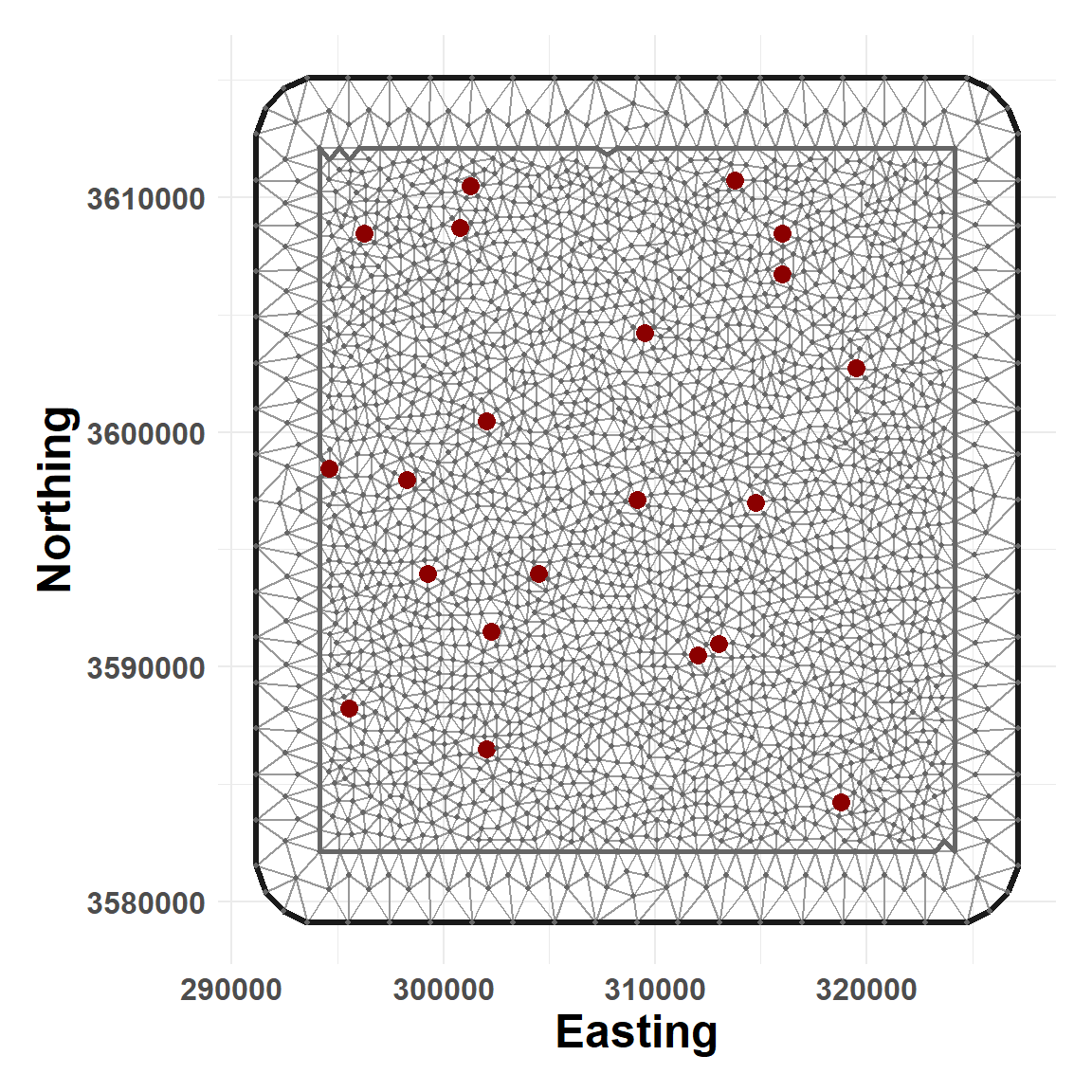

Combine data

Indexing all data to ensure all time steps (hours 1-6) are represented and inserting NA where data is unknown.

Hide code

comb_data_in <- replicate_data_timesteps(grid_raster = study_area$grid,
                                      farm_locs = study_area$farm_locs,
                                      concen_data = conc_melt,
                                      scale_concentration = 1e6,
                                      plume_model = plume_model,
                                      mesh = mesh.dom,
                                      max_hour = 6)

Mesh projection

Aligning, matching, or projecting data to the mesh.

Hide code

# flat prior based on study area width
width_m <- dim(study_area$grid)[1]*res(study_area$grid)[1]/3

sp_indices_dens <- project_to_mesh(comb_data = comb_data_in,
                                   prior.range=c(width_m, 0.01),
                                   prior.sigma=c(1, 0.01))

9 Organize Data

Organizing all model inputs as list() objects. This is needed because data within and between model tiers are different dimensions (i.e., won’t fit in a common data frame).

Individual particles

Organize tier 1 data for individual particles.

Hide code

comb_data_in$set_type <- as.integer(
  as.factor(comb_data_in$set)
)

dens.lst <- list(c(sp_indices_dens$field.sp.1,
                 list(intercept1 = 1)), 
                 list(height = comb_data_in[,"height"],
                      hour_step.1 = comb_data_in[,"hour"],
                      hour_step.2 = comb_data_in[,"hour"],
                      hour_step.3 = comb_data_in[,"hour"],
                      set_type = comb_data_in[,"set_type"])
                )

comb_data_in$Yd <- ifelse(comb_data_in$set == "particle", 1, 
                      ifelse(comb_data_in$set == "node", 0, NA)
)

dens.stk <- inla.stack(data = list(Y = comb_data_in$Yd),
                                 A = list(sp_indices_dens$A.mat, 1), 
                           effects = dens.lst,   
                               tag = "dens.0")

j.dens.stk <- inla.stack(data = list(Y = cbind(comb_data_in$Yd, NA), link = 1),
                                 A = list(sp_indices_dens$A.mat, 1), 
                           effects = dens.lst,   
                               tag = "dens.0")

Concentration

Organize tier 2 data for aggregate particle measures (concentration).

Hide code

conc.lst <- list(c(sp_indices_dens$field.sp.2,
                 list(intercept2 = 1)), 
                 list(x = comb_data_in[,"x"],
                      hour_step.1 = comb_data_in[,"hour"],
                      hour_step.2 = comb_data_in[,"hour"],
                      hour_step.3 = comb_data_in[,"hour"])
                )

comb_data_in$concen[comb_data_in$concen == 0] <- 1e-6 # gamma distributed

concen.stk <- inla.stack(data = list(Y = comb_data_in$concen),
                                 A = list(sp_indices_dens$A.mat, 1), 
                           effects = conc.lst,   
                               tag = "conc.0")

j.conc.stk <- inla.stack(data = list(Y = cbind(NA, comb_data_in$concen), link = 2),
                                 A = list(sp_indices_dens$A.mat, 1), 
                           effects = conc.lst,   
                               tag = "conc.0")

Combine Stacks

Combine the probability and and concentration data.

Hide code

joint.stack <- inla.stack(j.dens.stk, j.conc.stk)

10 Run Joint Spatiotemporal Model

The run_joint_spatiotemporal() is a wrapper function to facilitate model fitting with r-INLA. The model formula and execution can be viewed here: Model Details

Hide code

bin_gamma_model <- run_joint_spatiotemporal(field.sp.1 = sp_indices_dens$field.sp.1,
                                            field.sp.2 = sp_indices_dens$field.sp.2,
                                            spde_prior = sp_indices_dens$spde0,
                                            est.stk = joint.stack,
                                            verbose =TRUE)

# copy to OSF for others to access (~112mb)
osf_upload(osf_project_demo, path = here("local/assets/bg_model_2025-04-26.rds"))

Download pre-run from OSF

Hide code

osf_id <- osf_project_demo %>%
  osf_ls_files() %>%
  filter(name == "bg_model_2025-04-26.rds")

osf_download(osf_id,
             path = here("local/temp"),
             conflicts = "overwrite")

Read spatiotemporal model

Hide code

bin_gamma_model <- readRDS("local/temp/bg_model_2025-04-26.rds")

11 Model Results

Inspecting a few spatiotemporal model outputs.

Get Latent Fields

The get_spatial_rf() function spatial

Hide code

random_latent_field <- get_spatial_rf(model = bin_gamma_model,
                                      field_sp = sp_indices_dens$field.sp.1,
                                      raster_template = study_area$grid,
                                      mesh = mesh.dom
)

View Fields

Hide code

plot_latent_stack(rast_stack=random_latent_field,
                  farm_locs = study_area$farm_locs)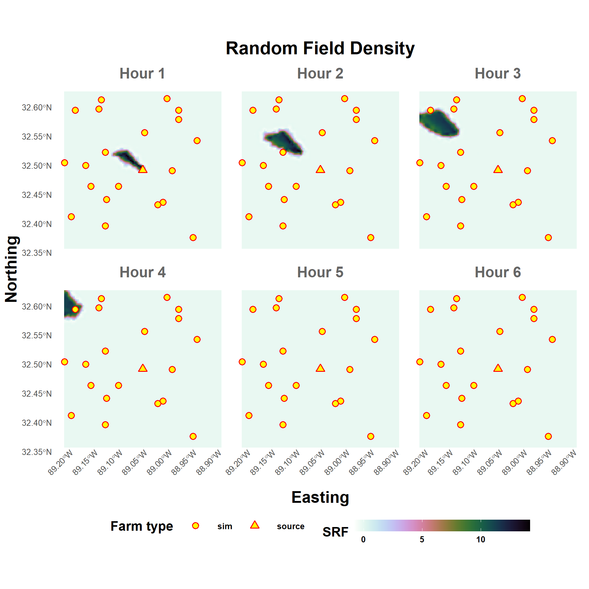

Particle Probabilty

Extracting the probability estimates for all locations in the study area.

Hide code

particle_probs <- extract_stmodel_estimates(model = bin_gamma_model,
                                            stack = joint.stack,
                                            stack_targ = "dens.0",
                                            match_data = comb_data_in,
                                            grid_label = "concen",
                                            raster_template = study_area$grid)

Hide code

plot_prob_stack(particle_probs)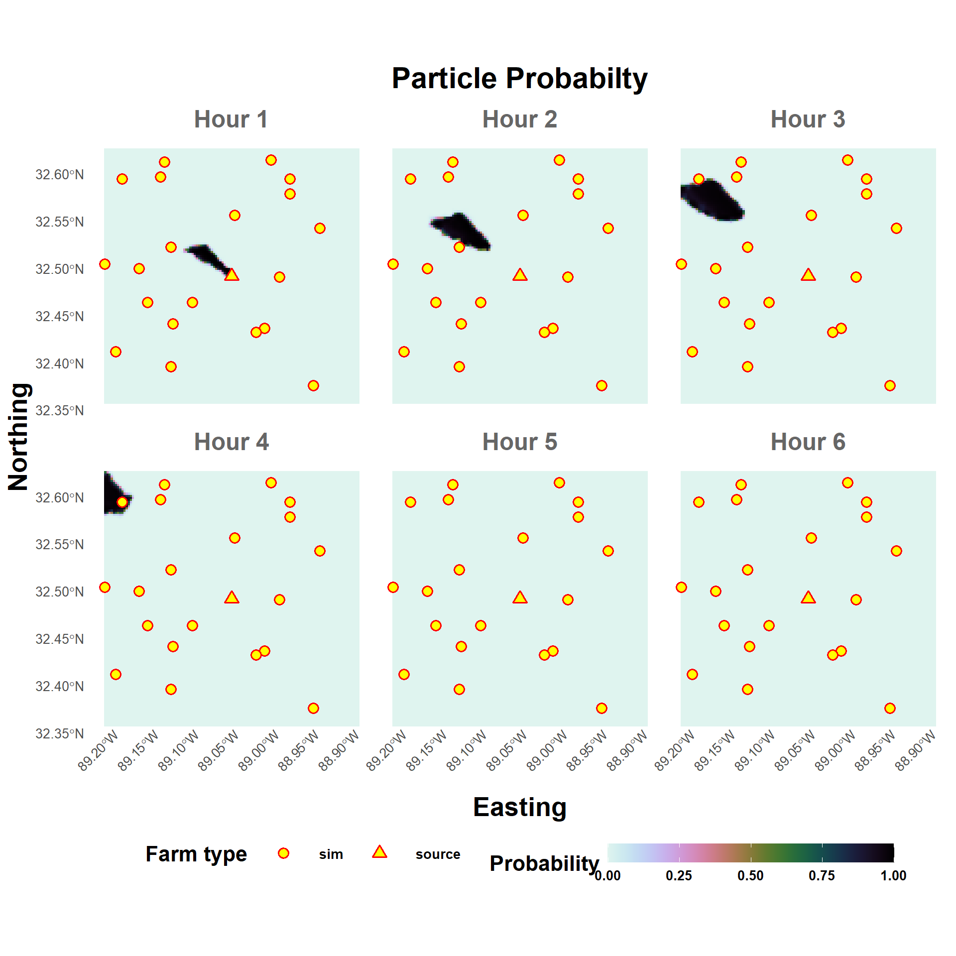

Particle Concentration

Extracting estimated concentrations for all locations in the study area.

Hide code

particle_conc <- extract_stmodel_estimates(model = bin_gamma_model,
                                            stack = joint.stack,
                                            stack_targ = "conc.0",
                                            match_data = comb_data_in,
                                            grid_label = "concen",
                                            raster_template = study_area$grid)

Hide code

plot_conc_stack(particle_conc)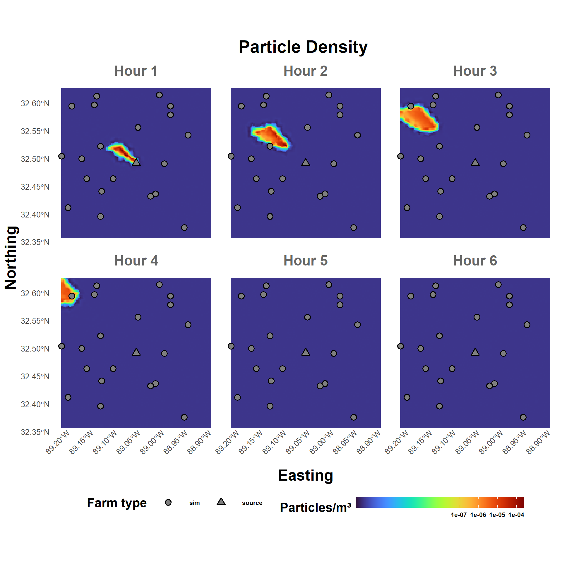

Optionally, can convert particle density to mass concentration (g/m3) using convert_particle_to_mass_concentration().

Hide code

mass_conc_stack <- particle_conc

values(mass_conc_stack) <- convert_particle_to_mass_concentration(concentration_particles_m3 = values(mass_conc_stack),
                                                                  pdiam_um = cfg$plume$pdiam,
                                                                  density_g_cm3 = cfg$plume$density,
                                                                  shape_factor = cfg$plume$shape_factor,
                                                                  output_units = "g/m3")

12 Farm Introduction Probability

Comparing particle probability estimates for simulated farm locations.

Hide code

farm_intro_probs <- extract_farm_estimates(model = bin_gamma_model,
                                           stack = joint.stack,
                                           stack_targ = "dens.0",
                                           match_data = comb_data_in)

Probability at farms

Hide code

farm_intro_probs$plot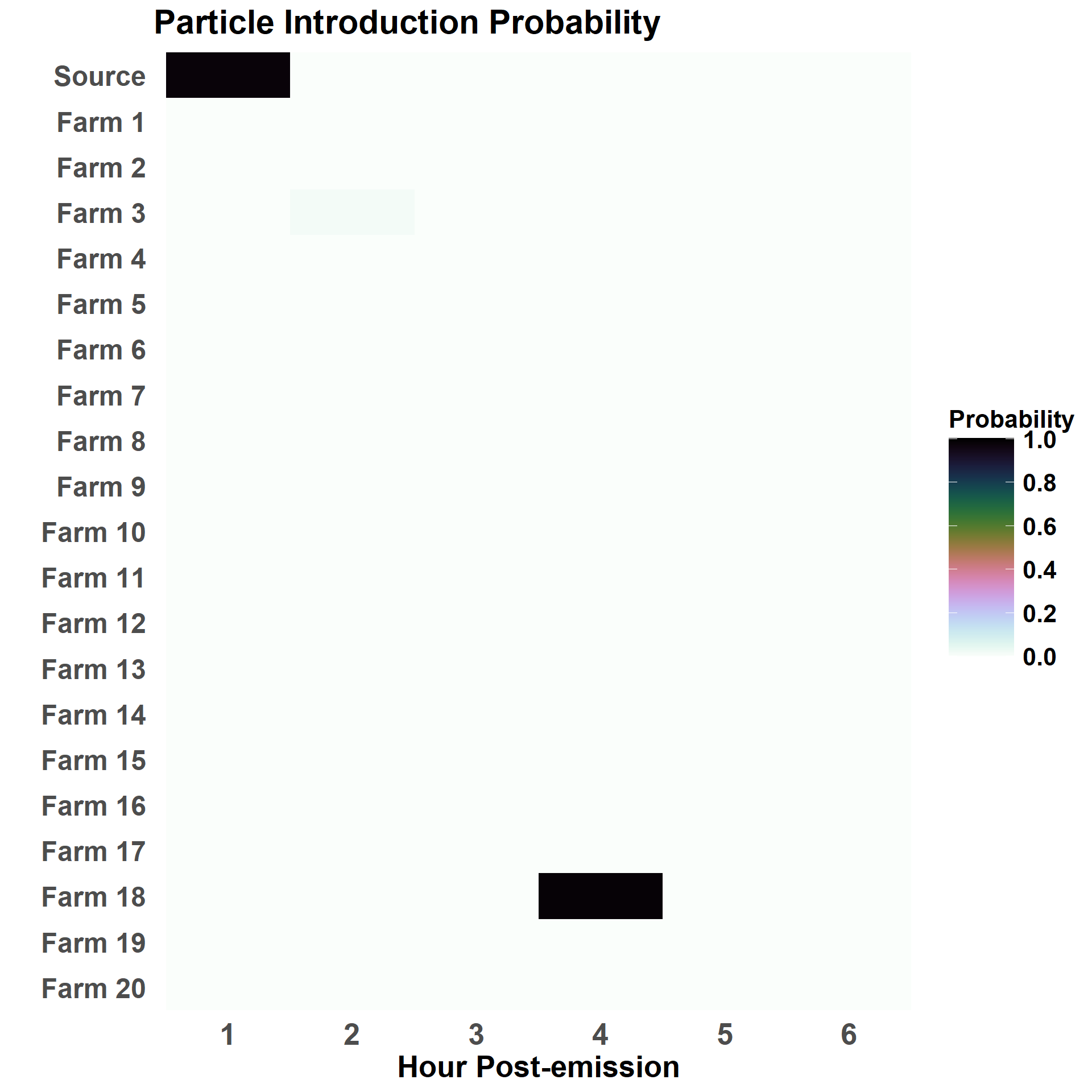

Filtering to simulated farms with at least a 50/% chance of particle occurrence.

Hide code

exposed_farms <- farm_intro_probs$table %>%
  filter(med >= 0.5 & name != "source_farm") # 50% chance or higher

exposed_farms

name	label	low	med	high	flock
farm_18	Farm 18	0.9823	0.9854	0.9868	22574

13 Secondary Outbreak

Given the high probability of particle introduction at a farm another than the source_farm, approximate how an outbreak might unfold based on that farm’s flock size, timeline of introduction, and other characteristics.

SEIR model for secondary ourbreak

Hide code

infect_date <- as_date(simulated_realease_dt)

intro_farm_args <- list(
  beta       = cfg$seir$beta,
  sigma      = 1 / cfg$seir$sigma,
  gamma      = 1 / cfg$seir$gamma,
  qV         = cfg$virus$qV,
  Vh         = cfg$poultry$house_vol,
  Q          = cfg$poultry$Q_m3_h * 24,
  lamd       = log(2) / halflife,
  flock_size = exposed_farms$flock, # flock size where virus introduced
  Ei         = cfg$seir$Ei,
  Ii         = cfg$seir$Ii,
  Ri         = cfg$seir$Ri,
  Vi         = cfg$seir$Vi,
  sim_days   = cfg$seir$sim_days,
  infect_date = infect_date # infection same day as emission (only hours difference)
)

seir_exposed_farm <- do.call(model_seir_shedding, intro_farm_args)

Outbreak at exposed farm. For rand_detect_day, assuming detection occurs 5 to 20 days after outbreaks start. That is, when workers notice that death rates are exceeding the normal background rate.

Hide code

set.seed(1976)
rand_detect_day <- round(runif(1, 5, 20),0)
detection_date <- infect_date + days(rand_detect_day)

View outbreak dynamics

Hide code

plot_ode_shed_dynamics(seir_exposed_farm, date_axis = TRUE, vline = detection_date, vline_text = "Detection")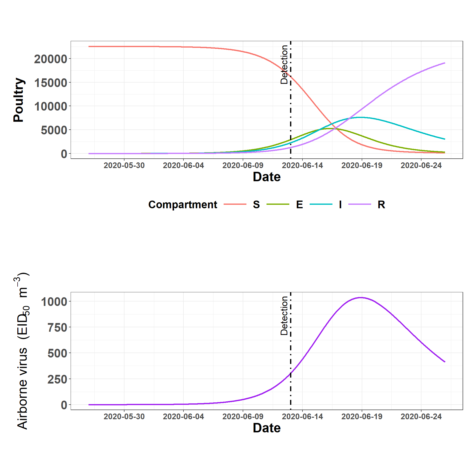

14 Write Simulation Result

Recording outbreak simulation info to be used in downstream analysis.

Hide code

farms_wgs84 <- project(study_area$farm_locs, "EPSG:4326") # long/lat

simulation_keep <- as.data.frame(farms_wgs84, geom="xy") %>%
  mutate(outbreak = if_else(name == exposed_farms$name, detection_date,
         if_else(name == "source_farm", sim_dates$release_date, NA)))

Write copies locally and on OSF

Hide code

# local copy
write.csv(simulation_keep, here("local/assets/demo_outbreak_sim_2025-04-28.csv"))

# copy to OSF for others to access
osf_upload(osf_project_demo, path = here("local/assets/demo_outbreak_sim_2025-04-28.csv"))

15 Closing

This script simulated a pathogen plume from a source farm location followed secondary outbreaks at other farms downwind. Next, the results here are analysed in the script linked here to determine if that outbreak can be traced back to the original source farm.