Between-Farm Transmission

Simulation of an FMDV spread between farms

Description

The challengeABM package includes the simulate_net_model() function that accepts a networkis calibrated to exhibit the same within-host virus dynamics as the simulate_room_to_room() function uses for laboratory based animal experiments. At simulation start, cattle (agents) are populated to a common area with a specified number of FMDV infected individuals. On simulation hour 1, cattle begin making random contact with each other at a specified hourly rate to show homogeneous mixing.

Depending on the quantity of virus in the donor cattle and chance contacts, they may or may not infect others. The quantity of virus in nasal passages and in blood serum has been calibrated to match the experimental study described in the analysis with parameters recorded in the default_herd_config.yaml configuration file that is available with this script.

challengeABM Package

Simulation code is available here: challengeABM. The GitHub site includes an Overview, Design concepts, Details document.

Hide code

# library(remotes)
# remotes::install_github("geoepi/challengeABM")

library(challengeABM)

Read Configuration File

Hide code

config_file <- read_yaml(here("config/base_config_fmdv.yaml"))

Generate Network

The generate_farm_network() function is used to create a graph network representing the spatial relationships between farms and number of cattle in each. Nodes in the network represent farms and edges are proportional to the distance between those farms. The returned list() includes a randomized $graph network object and a $farm_df data frame with the farm labels and cattle number.

Using parameters in the configuration file:

Randomized spatial arrangement

Hide code

net <- generate_farm_network(config_file)

plot_base_network(net$graph)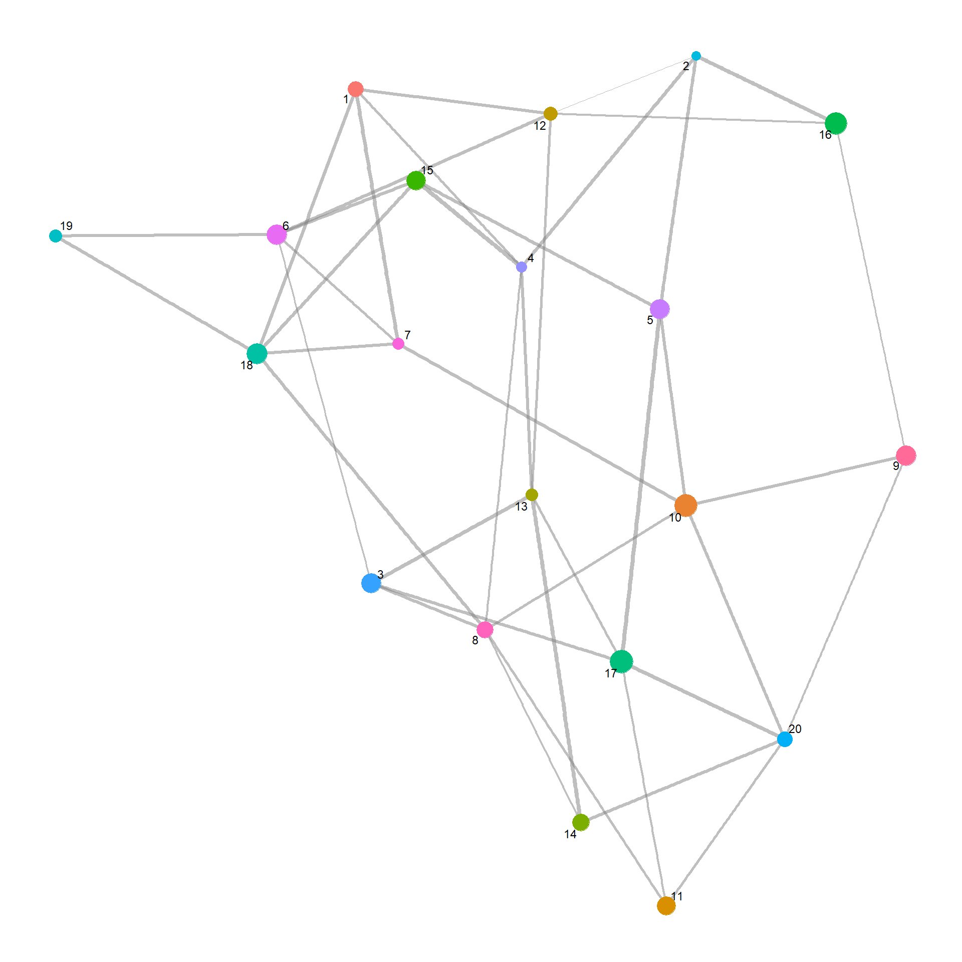

Randomized number of cattle

Hide code

# dimensions
dim(net$farm_df)

[1] 20  3

Hide code

# peek at data
head(net$farm_df)

farm_id	node_id	herd_size
farm_1	1	277
farm_2	2	107
farm_3	3	572
farm_4	4	119
farm_5	5	552
farm_6	6	598

Hide code

# cattle numbers
range(net$farm_df$herd_size)

[1] 107 935

Or alternatively using overrides:

Hide code

net_2 <- generate_farm_network(config_file,
                               n_farms = 100,
                               graph_type = "smallworld",
                               herd_size_range = c(1000, 5000),
                               seed = 12345)

plot_base_network(net_2$graph)

Hide code

# dimensions
dim(net_2$farm_df)

[1] 100   3

Hide code

# peek at data
head(net_2$farm_df)

farm_id	node_id	herd_size
farm_1	1	2881
farm_2	2	2152
farm_3	3	2270
farm_4	4	1432
farm_5	5	4383
farm_6	6	2880

Hide code

# cattle numbers
range(net_2$farm_df$herd_size)

[1] 1043 4955

Run Simulation

The simulate_net_model() functions accepts the network and disease parameters from the config file and runs the simulation. This parameterization takes 3-5 minutes to run, therefore a copy is saved for reload.

Hide code

model_result <- simulate_net_model(net, config_file)

saveRDS(model_result, here("local/demo/model_result_2025-06-13.rds"))

Download saved copy from OSF

Hide code

osf_id <- osf_project_demo %>%
  osf_ls_files() %>%
  filter(name == "model_result_2025-06-13.rds") # file to download

osf_download(osf_id,
             path = here("local/temp"), # where to save
             conflicts = "overwrite")

name	id	local_path	meta
model_result_2025-06-13.rds	684cbc31fea3288c3ab687ad	local/temp/model_result_2025-06-13.rds	model_result_2025-06-13.rds , file , /684cbc31fea3288c3ab687ad , 4172117 , osfstorage , /model_result_2025-06-13.rds , 1749859377 , 1749859377 , 274f06b6116b3d5bfe1088de8649938f , de11d00cab4e4f25dc259ee39b7567bfb0785b581447460e5f060a45fb15f0bf , 0 , TRUE , 1 , FALSE , https://api.osf.io/v2/files/684cbc31fea3288c3ab687ad/ , https://files.osf.io/v1/resources/qf2wr/providers/osfstorage/684cbc31fea3288c3ab687ad , https://files.osf.io/v1/resources/qf2wr/providers/osfstorage/684cbc31fea3288c3ab687ad , https://files.osf.io/v1/resources/qf2wr/providers/osfstorage/684cbc31fea3288c3ab687ad , https://osf.io/download/684cbc31fea3288c3ab687ad/ , https://mfr.osf.io/render?url=https%3A%2F%2Fosf.io%2Fdownload%2F684cbc31fea3288c3ab687ad%2F%3Fdirect%26mode%3Drender, https://osf.io/qf2wr/files/osfstorage/684cbc31fea3288c3ab687ad , https://api.osf.io/v2/files/684cbc31fea3288c3ab687ad/ , https://api.osf.io/v2/files/684cb2aed0a256104638874a/ , 684cb2aed0a256104638874a , files , https://api.osf.io/v2/files/684cbc31fea3288c3ab687ad/versions/ , https://api.osf.io/v2/nodes/qf2wr/ , qf2wr , nodes , https://api.osf.io/v2/nodes/qf2wr/ , nodes , nodes , qf2wr , https://api.osf.io/v2/files/684cbc31fea3288c3ab687ad/cedar_metadata_records/

Hide code

# read save file to environment
model_result <- readRDS(here("local/temp/model_result_2025-06-13.rds"))

Examine returned object. The returned object is a nested list, with dataframes for each farm and animal at each time step.

Hide code

length(model_result)

[1] 3

Hide code

names(model_result)

[1] "farm_status"    "movement_log"   "quarantine_log"

Hide code

names(model_result$farm_status)

[1] "herd_agents" "herd_states" "quarantined"

Hide code

names(model_result$farm_status$herd_agents)

 [1] "farm_1"  "farm_2"  "farm_3"  "farm_4"  "farm_5"  "farm_6"  "farm_7" 
 [8] "farm_8"  "farm_9"  "farm_10" "farm_11" "farm_12" "farm_13" "farm_14"
[15] "farm_15" "farm_16" "farm_17" "farm_18" "farm_19" "farm_20"

Hide code

names(model_result$farm_status$herd_agents$farm_1)

 [1] "id"                              "infection_status"               
 [3] "infect_agent"                    "is_donor"                       
 [5] "virus_nasal"                     "virus_serum"                    
 [7] "score_t"                         "nasal_threshold"                
 [9] "serum_threshold"                 "infect_threshold"               
[11] "dose"                            "infectious_t"                   
[13] "growth_rate_nasal"               "growth_rate_serum"              
[15] "clearance_rate"                  "stochastic_noise"               
[17] "exponential_factor"              "inflection_point_nasal"         
[19] "inflection_point_serum"          "inflection_point_absolute_nasal"
[21] "inflection_point_absolute_serum" "growth_cease"                   
[23] "nasal_ccap"                      "serum_ccap"                     
[25] "infection_time"                  "score"                          
[27] "recovery_time"                   "has_recovered"                  
[29] "infector_id"                     "preclin_onset"                  
[31] "preclin_dur"                     "clinical_dur"                   
[33] "transmitter_state"               "time_since_infection"           
[35] "state"                          

Extract Stats

Pulling a few statistics from the simulation using extract_net_simulation_summary(). Note that functions such as calculate_R0_from_network() are available to calculate stats from a series of literately run models.

Basic stats:
- R_farm: Farm-level reproduction estimated by outgoing node edges in network.
- outbreak_farms: Total number of farms with outbreaks in this demo simulation.
- first_infection_time: Time when first infection was detected.
- total_infected_at_first: Total animals infected at time first animal was detected (i.e., some undetected).
- total_infected_animals: Total infected animals over course of outbreak.

Hide code

extract_net_simulation_summary(model_result)

R_farm	outbreak_farms	first_infection_time	total_infected_at_first	total_infected_animals
3.285714	14	14	2	7775

Animation

Viewing between farm disease spread.

Hide code

animate_spread(net=net,
               farm_states = model_result$farm_status$herd_states, 
               move_df = dplyr::bind_rows(model_result$movement_log),
               output_file = here("images/spread.gif")
               )

Hide code

knitr::include_graphics(here("images/spread.gif"))